Simulating DeLosh 1997
Simulation
ALM
EXAM
R
Code
#https://nrennie.rbind.io/blog/2022-06-06-creating-flowcharts-with-ggplot2/
inNodes <- seq(1,6,1) %>% as.integer()
outNodes <- seq(300,1000,50)%>% as.integer()

stim <- "Stim"
resp <- "Response"
inFlow <- tibble(expand.grid(from=stim,to=inNodes)) %>% mutate_all(as.character)
outFlow <- tibble(expand.grid(from=outNodes,to=resp)) %>% mutate_all(as.character)

gd <- tibble(expand.grid(from=inNodes,to=outNodes)) %>% mutate_all(as.character) %>%
  rbind(inFlow,.) %>% rbind(.,outFlow)

g = graph_from_data_frame(gd,directed=TRUE)
coords2=layout_as_tree(g)
colnames(coords2)=c("y","x")
odf <- as_tibble(coords2) %>%
  mutate(label=vertex_attr(g,"name"),
         type=c("stim",rep("Input",length(inNodes)),rep("Output",length(outNodes)),"Resp"),
         x=x*-1) %>%
  mutate(y=ifelse(type=="Resp",0,y),xmin=x-.05,xmax=x+.05,ymin=y-.35,ymax=y+.35)

plot_edges = gd %>% mutate(id=row_number()) %>%
  pivot_longer(cols=c("from","to"),names_to="s_e",values_to=("label")) %>%
                 mutate(label=as.character(label)) %>%
  group_by(id) %>%
  mutate(weight=sqrt(rnorm(1,mean=0,sd=10)^2)/10) %>%
  left_join(odf,by="label") %>%
  mutate(xmin=xmin+.02,xmax=xmax-.02)

ggplot() + geom_rect(data = odf,
            mapping = aes(xmin = xmin, ymin = ymin,
                          xmax = xmax, ymax = ymax,
                          fill = type, colour = type),alpha = 0.5) +
  geom_text(data=odf,aes(x=x,y=y,label=label,size=3)) +
  geom_path(data=plot_edges,mapping=aes(x=x,y=y,group=id,alpha=weight)) +
theme_void() + theme(legend.position = "none") 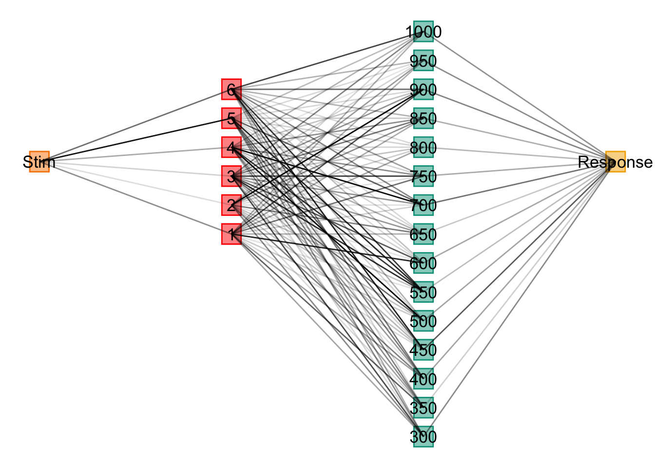
Code
linear_function <- function(x) 2.2 * x + 30
exponential_function <- function(x) 200 * (1 - exp(-x/25))
quadratic_function <- function(x) 210 - (x - 50)^2 / 12

extrapLines <- list(geom_vline(xintercept=30,color="black",alpha=.4,linetype="dashed"),
                    geom_vline(xintercept=70,color="black",alpha=.4,linetype="dashed"))

linear_plot <- ggplot(deLosh_data$human_data_linear, aes(x, y)) +
    geom_point(shape=1) + stat_function(fun = linear_function, color = "black") +
  labs(y="Response Magnitude", title="Linear Function",x="") + extrapLines

exponential_plot <- ggplot(deLosh_data$human_data_exp, aes(x, y)) +
  geom_point(aes(shape = "Observed", color = "Observed"),shape=1) +
  stat_function(aes(color = "True Function"),fun = exponential_function, geom="line")+
  labs(x="Stimulus Magnitude", title="Exponential Function",y="")  +
  extrapLines +
  scale_shape_manual(values = c(1)) +
  scale_color_manual(values = c("Observed" = "black", "True Function" = "black")) +
  theme(legend.title = element_blank(), legend.position="top") +
  guides(color = guide_legend(override.aes = list(shape = c(1, NA),
                                                  linetype = c(0, 1))))

quadratic_plot <- ggplot(deLosh_data$human_data_quad, aes(x = x, y = y)) +
  geom_point( shape = 1) +
  stat_function( fun = quadratic_function, geom = "line") +
  labs(title="Quadratic Function",x="",y="") + extrapLines

linear_plot + exponential_plot + quadratic_plot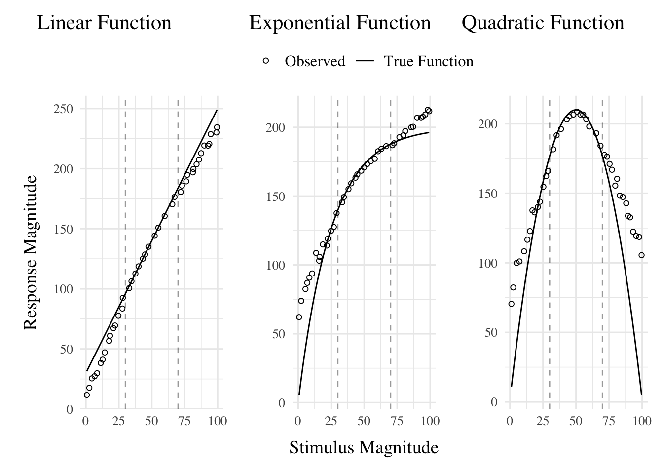
ALM Definition
Input Activation
\[ a_i(X)=\exp \left|-\gamma \cdot\left[X-X_i\right]^2\right| \]
Output activation
\[ o_j(X)=\Sigma_{i=1, M} w_{j i} \cdot a_i(X) \]
Output Probability
\[ P\left[Y_j \mid X\right]=o_j(X) / \Sigma_{k=1, L} o_k(X) \]
Mean Response
\[ m(X)=\Sigma_{j=1, L} Y_j \cdot P\left[Y_j \mid X\right] \]
Feedback Signal
\[ f_j(Z)=e^{-c\cdot(Z-Y_j)^2} \]
Weight Updates
\[ w_{ji}(t+1)=w_{ji}(t)+\alpha \cdot {f_i(Z(t))-O_j(X(t))} \cdot a_i(X(t)) \]
Input node actvation
\[ P[X_i|X] = \frac{a_i(X)}{\\sum_{k=1}^Ma_k(X)} \]
Slope Computation
\[ E[Y|X_i]=m(X_i) + \bigg[\frac{m(X_{i+1})-m(X_{i-1})}{X_{i+1} - X_{i-1}} \bigg]\cdot[X-X_i] \]
Generate Response
Code
##| code-fold: show
#| code-summary: "Toggle Code"
alm.response <- function(input = 1, c, input.layer, output.layer,weight.mat) {
  input.activation <- exp(-c * (input.layer - input)^2) / sum(exp(-c * (input.layer - input)^2))
  output.activation <- weight.mat %*% input.activation
  output.probability <- output.activation / sum(output.activation)
  mean.response <- sum(output.layer * output.probability)
  list(mean.response = mean.response, input.activation = input.activation, output.activation = output.activation)
}
Update Weights Based on Feedback
Toggle Code
alm.update <- function(corResp, c, lr, output.layer, input.activation, output.activation, weight.mat) {
  fz <- exp(-c * (output.layer - corResp)^2)
  teacherSignal <- (fz - output.activation) * lr
  wChange <- teacherSignal %*% t(input.activation)
  weight.mat <- weight.mat + wChange
  weight.mat[weight.mat < 0] = 0
  return(weight.mat)
}

alm.trial <- function(input, corResp, c, lr, input.layer, output.layer, weight.mat) {
  alm_resp <- alm.response(input, c, input.layer,output.layer, weight.mat)
  updated_weight.mat <- alm.update(corResp, c, lr, output.layer, alm_resp$input.activation, alm_resp$output.activation, weight.mat)
  return(list(mean.response = alm_resp$mean.response, weight.mat = updated_weight.mat))
}
Exam Generalization
Toggle Code
exam.response <- function(input, c, trainVec, input.layer = INPUT_LAYER_DEFAULT,output.layer = OUTPUT_LAYER_DEFAULT, weight.mat) {
  nearestTrain <- trainVec[which.min(abs(input - trainVec))]
  aresp <- alm.response(nearestTrain, c, input.layer = input.layer,output.layer = OUTPUT_LAYER_DEFAULT,weight.mat)$mean.response

  xUnder <- ifelse(min(trainVec) == nearestTrain, nearestTrain, trainVec[which(trainVec == nearestTrain) - 1])
  xOver <- ifelse(max(trainVec) == nearestTrain, nearestTrain, trainVec[which(trainVec == nearestTrain) + 1])

  mUnder <- alm.response(xUnder, c, input.layer = input.layer, output.layer, weight.mat)$mean.response
  mOver <- alm.response(xOver, c, input.layer = input.layer,output.layer, weight.mat)$mean.response

  exam.output <- round(aresp + ((mOver - mUnder) / (xOver - xUnder)) * (input - nearestTrain), 3)
  exam.output
}
Simulation Functions
Code
# simulation function
alm.sim <- function(dat, c, lr, input.layer = INPUT_LAYER_DEFAULT, output.layer = OUTPUT_LAYER_DEFAULT) {
  weight.mat <- matrix(0.00, nrow = length(output.layer), ncol = length(input.layer))
  xt <- dat$x
  n <- nrow(dat)
  st <- numeric(n) # Initialize the vector to store mean responses
  for(i in 1:n) {
    trial <- alm.trial(dat$x[i], dat$y[i], c, lr, input.layer, output.layer, weight.mat)
    weight.mat <- trial$weight.mat
    st[i] <- trial$mean.response
  }
  dat <- dat %>% mutate(almResp = st)
  return(list(d = dat, wm = weight.mat, c = c, lr = lr))
}


simOrganize <- function(simOut) {
  dat <- simOut$d
  weight.mat <- simOut$wm
  c <- simOut$c
  lr <- simOut$lr
  trainX <- unique(dat$x)

  almResp <- generate.data(seq(0,100,.5), type = first(dat$type)) %>% rowwise() %>%
    mutate(model = "ALM", resp = alm.response(x, c, input.layer = INPUT_LAYER_DEFAULT,output.layer = OUTPUT_LAYER_DEFAULT, weight.mat = weight.mat)$mean.response)

  examResp <- generate.data(seq(0,100,.5), type = first(dat$type)) %>% rowwise() %>%
    mutate(model = "EXAM", resp = exam.response(x, c, trainVec = trainX, input.layer = INPUT_LAYER_DEFAULT,output.layer = OUTPUT_LAYER_DEFAULT, weight.mat))

  organized_data <- bind_rows(almResp, examResp) %>%
    mutate(type = first(dat$type),
           error = abs(resp - y),
           c = c,
           lr = lr,
           type = factor(type, levels = c("linear", "exponential", "quadratic")),
           test_region = ifelse(x %in% trainX, "train",
                                ifelse(x > min(trainX) & x < max(trainX), "interpolate", "extrapolate")))
  organized_data
}


generateSimData <- function(density, envTypes, noise) {
  reps <- 200 / length(trainingBlocks[[density]])
  map_dfr(envTypes, ~
            generate.data(rep(trainingBlocks[[density]], reps), type = .x, noise)) |>
    group_by(type) |>
    mutate(block = rep(1:reps, each = length(trainingBlocks[[density]])),
           trial=seq(1,200))
}

simulateAll <- function(density,envTypes, noise, c = .2, lr = .2) {
  trainMat <- generateSimData(density, envTypes, noise)
  trainData <- map(envTypes, ~ alm.sim(trainMat %>% filter(type == .x), c = c, lr = lr))
  assign(paste(density),list(train=trainData, test=map_dfr(trainData, simOrganize) %>% mutate(density = density)))
}
Simulate Training and Testing
Code
envTypes <- c("linear", "exponential", "quadratic")
densities <- c("low", "med", "high")
noise=0
INPUT_LAYER_DEFAULT <- seq(0, 100, 0.5)
OUTPUT_LAYER_DEFAULT <- seq(0, 250, 1)

c = 1.4
lr=.8

results <- map(densities, ~ simulateAll(.x, envTypes, noise, c, lr)) |>
  set_names(densities)

trainAll <- results %>%
  map_df(~ map_df(.x$train, pluck, "d"), .id = "density") |>
  mutate(stage=as.numeric(cut(trial,breaks=20,labels=seq(1,20))),
         dev=sqrt((y-almResp)^2),
         density=factor(density,levels=c("low","med","high")),
         type=factor(type,levels=c("linear","exponential","quadratic"))) |>
  dplyr::relocate(density,type,stage)

simTestAll <- results |> map("test") |> bind_rows() |>
  group_by(type,density,model) %>%
  mutate(type=factor(type,levels=c("linear","exponential","quadratic")),
         density=factor(density,levels=c("low","med","high"))) %>%
  dplyr::relocate(density,type,test_region)
Training Data
Code
trainAll %>% ggplot(aes(x=block,y=dev,color=type)) + stat_summary(geom="line",fun=mean,alpha=.4)+
  stat_summary(geom="point",fun=mean,alpha=.4)+
  stat_summary(geom="errorbar",fun.data=mean_cl_normal,alpha=.4)+facet_wrap(~density, scales="free_x")
Predictions for Generalization
Code
simTestAll %>% ggplot(aes(x=x,y=y)) +
  geom_point(aes(x=x,y=resp,shape=model,color=model),alpha=.7,size=1) +
  geom_line(aes(x=x,y=y),alpha=.4)+
  geom_point(data=simTestAll %>% filter(test_region=="train"),aes(x=x,y=y),color="black",size=1,alpha=1) +
  facet_grid(density~type) +
  theme_bw() + theme(legend.position="bottom")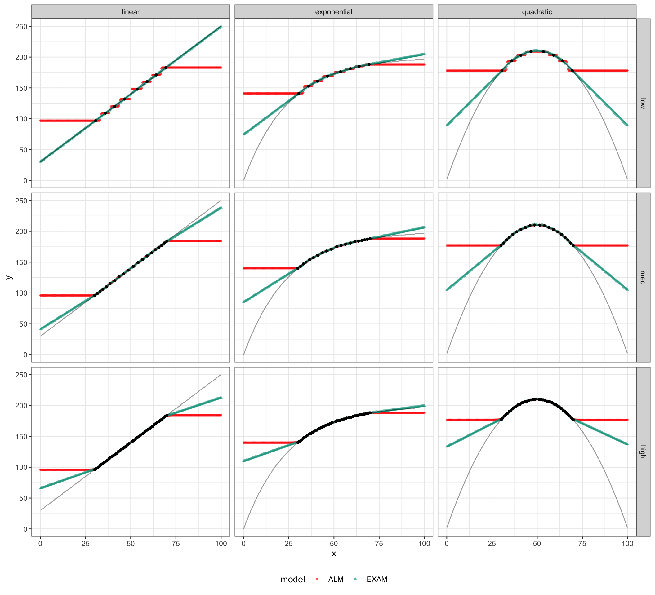
Collpasing Across Density Levels gives us:
Code
simTestAll %>% group_by(type,model,x,y) %>% summarise(resp=mean(resp))  %>% ggplot(aes(x=x,y=y)) +
  geom_point(aes(x=x,y=resp,shape=model,color=model),alpha=.7,size=1) +
  geom_line(aes(x=x,y=y),alpha=.4)+
  facet_grid(~type) +
  theme_bw() + theme(legend.position="bottom")
Table
| Model & Definition | R Code |
|---|---|
| \(a_i(X)=\exp \left|-\gamma \cdot\left[X-X_i\right]^2\right|\) | exp(-c * (input.layer - input)^2) |
| \(o_j(X)=\Sigma_{i=1, M} w_{j i} \cdot a_i(X)\) | weight.mat %*% input.activation |
| \(P\left[Y_j \mid X\right]=o_j(X) / \Sigma_{k=1, L} o_k(X)\) | output.activation / sum(output.activation) |
| \(m(X)=\Sigma_{j=1, L} Y_j \cdot P\left[Y_j \mid X\right]\) | sum(output.layer * output.probability) |
| \(f_j(Z)=e^{-c\cdot(Z-Y_j)^2}\) | exp(-c * (output.layer - corResp)^2) |
| \(w_{ji}(t+1)=w_{ji}(t)+\alpha \cdot {f_i(Z(t))-O_j(X(t))} \cdot a_i(X(t)\) | lr *(fz - output.activation) %*% t(input.activation) |
| \(E[Y|X_i]=m(X_i) + \bigg[\frac{m(X_{i+1})-m(X_{i-1})}{X_{i+1} - X_{i-1}} \bigg]\cdot[X-X_i]\) | trainVec[which.min(abs(input - trainVec))]; xUnder <- ...; xOver <- ...; mUnder <- ...; mOver <- ...; exam.output <- round(aresp + ((mOver - mUnder) / (xOver - xUnder)) * (input - nearestTrain), 3) |