The major adjustment of Experiment 3 is for participants to receive ordinal feedback during training, in contrast to the continuous feedback of the prior experiments. After each training throw, participants are informed whether a throw was too soft, too hard, or correct (i.e. within the target velocity range). All other aspects of the task and design are identical to Experiments 1 and 2. We utilized the order of training and testing bands from both of the prior experiments, thus assigning participants to both an order condition (Original or Reverse) and a training condition (Constant or Varied). Participants were once again recruited from the online Indiana University Introductory Psychology Course pool. Following exclusions, 195 participants were included in the final analysis, n=51 in the Constant-Original condition, n=59 in the Constant-Reverse condition, n=39 in the Varied-Original condition, and n=46 in the Varied-Reverse condition.
Table 1: Experiment 3 - End of training performance. The Intercept represents the average of the baseline (constant condition), and the conditVaried coefficient reflects the difference between the constant and varied groups. A larger positive coefficient indicates a greater deviation (lower accuracy) for the varied group.
Term
Estimate
95% CrI Lower
95% CrI Upper
pd
Intercept
121.86
109.24
134.60
1.00
conditVaried
64.93
36.99
90.80
1.00
bandOrderReverse
1.11
-16.02
18.16
0.55
conditVaried:bandOrderReverse
-77.02
-114.16
-39.61
1.00
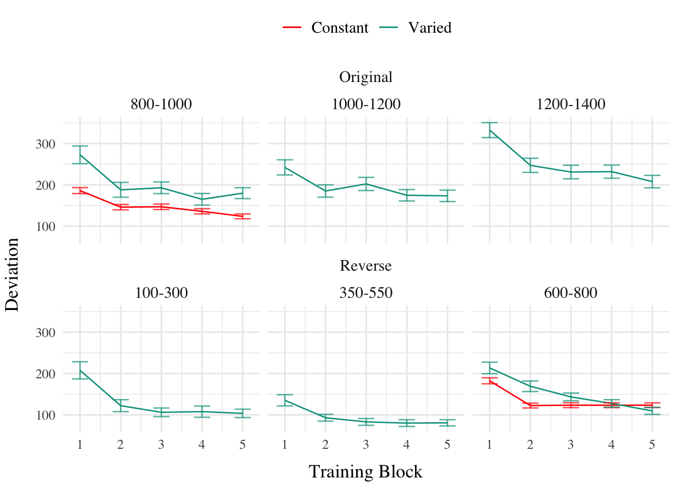
Training. Figure 1 displays the average deviations from the target band across training blocks, and Table 1 shows the results of the Bayesian regression model predicting the deviation from the common band at the end of training (600-800 for reversed order, and 800-1000 for original order conditions). The main effect of training condition is significant, with the varied condition showing larger deviations ( \(\beta\) = 64.93, 95% CrI [36.99, 90.8]; pd = 100%). The main effect of band order is not significant \(\beta\) = 1.11, 95% CrI [-16.02, 18.16]; pd = 55.4%, however the interaction between training condition and band order is significant, with the varied condition showing greater accuracy in the reverse order condition ( \(\beta\) = -77.02, 95% CrI [-114.16, -39.61]; pd = 100%).
Code
p1<-trainE3|>ggplot(aes(x =Trial_Bin, y =dist, color =condit))+stat_summary(geom ="line", fun =mean)+stat_summary(geom ="errorbar", fun.data =mean_se, width =.4, alpha =.7)+ggh4x::facet_nested_wrap(~bandOrder*vb,ncol=3)+scale_x_continuous(breaks =seq(1, nbins+1))+theme(legend.title=element_blank())+labs(y ="Deviation", x="Training Block")#ggsave(here("Assets/figs/e3_train_deviation.png"), p1, width = 9, height = 8,bg="white")p1
Figure 1: E3. Deviations from target band during testing without feedback stage.
Table 2: Experiment 3 testing accuracy. Main effects of condition and band type (training vs. extrapolation), and the interaction between the two factors. The Intercept represents the baseline condition, (constant training; trained bands & original order), and the remaining coefficients reflect the deviation from that baseline. Positive coefficients thus represent worse performance relative to the baseline, - and a positive interaction coefficient indicates disproportionate deviation for the varied condition or reverse order condition.
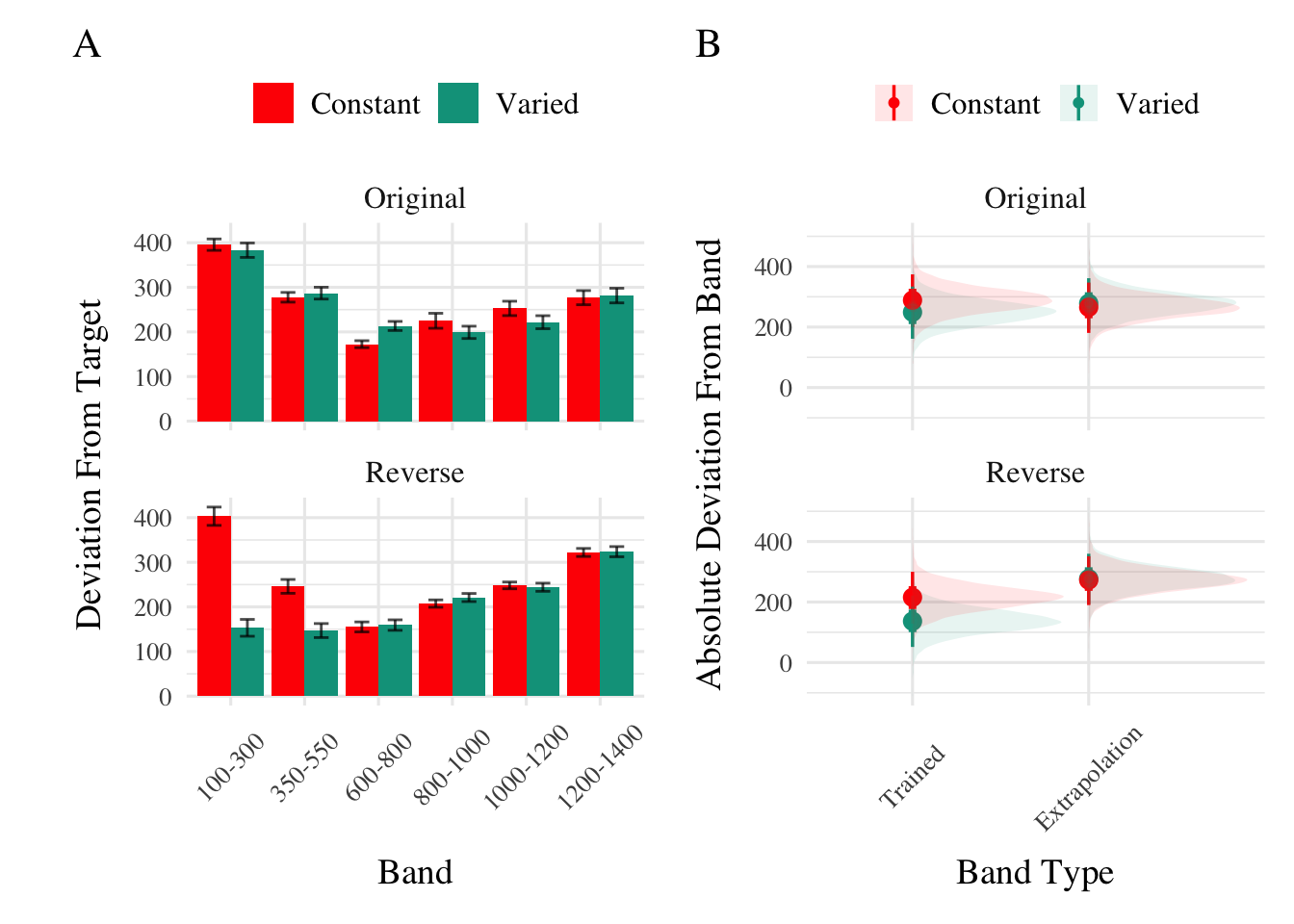
Testing Accuracy.Table 2 presents the results of the Bayesian mixed efects model predicting absolute deviation from the target band during the testing stage. There was no significant main effect of training condition,\(\beta\) = -40.19, 95% CrI [-104.68, 23.13]; pd = 89.31%, or band type,\(\beta\) = -23.35, 95% CrI [-57.28, 10.35]; pd = 91.52%. However the effect of band order was significant, with the reverse order condition showing lower deviations, \(\beta\) = -73.72, 95% CrI [-136.69, -11.07]; pd = 98.89%. The interaction between training condition and band type was also significant \(\beta\) = 52.66, 95% CrI [14.16, 90.23]; pd = 99.59%, with the varied condition showing disproprionately large deviations on the extrapolation bands compared to the constant group. There was also a significant interaction between band type and band order, \(\beta\) = 80.69, 95% CrI [30.01, 130.93]; pd = 99.89%, such that the reverse order condition showed larger deviations on the extrapolation bands. No other interactions were significant.
Code
condEffects<-function(m,xvar){m|>ggplot(aes(x ={{xvar}}, y =.value, color =condit, fill =condit))+stat_dist_pointinterval()+stat_halfeye(alpha=.1, height=.5)+theme(legend.title=element_blank(),axis.text.x =element_text(angle =45, hjust =0.5, vjust =0.5))}pe3td<-testE3|>ggplot(aes(x =vb, y =dist,fill=condit))+stat_summary(geom ="bar", position=position_dodge(), fun =mean)+stat_summary(geom ="errorbar", position=position_dodge(.9), fun.data =mean_se, width =.4, alpha =.7)+facet_wrap(~bandOrder,ncol=1)+theme(legend.title=element_blank(),axis.text.x =element_text(angle =45, hjust =0.5, vjust =0.5))+labs(x="Band", y="Deviation From Target")pe3ce<-bmtd3|>emmeans(~condit*bandOrder*bandType)|>gather_emmeans_draws()|>condEffects(bandType)+labs(y="Absolute Deviation From Band", x="Band Type")+facet_wrap(~bandOrder,ncol=1)p2<-pe3td+pe3ce+plot_annotation(tag_levels='A')#ggsave(here::here("Assets/figs", "e3_test-dev.png"), p2, width=9, height=8, bg="white")p2
Figure 2: Experiment 3 Testing Accuracy. A) Deviations from target band during testing without feedback stage. B) Conditional effect of condition (Constant vs. Varied) and testing band type (training vs. extrapolation) on testing accuracy. Error bars represent 95% confidence intervals.
Table 3: Experiment 3. Bayesian Mixed Model Predicting Vx as a function of condition (Constant vs. Varied) and Velocity Band. The Intercept represents the baseline condition (constant training & original order), and the Band coefficient represents the linear slope for the baseline condition.
Term
Estimate
95% CrI Lower
95% CrI Upper
pd
Intercept
601.83
504.75
699.42
1.00
conditVaried
12.18
-134.94
162.78
0.56
bandOrderReverse
13.03
-123.89
144.67
0.58
Band
0.49
0.36
0.62
1.00
conditVaried:bandOrderReverse
-338.15
-541.44
-132.58
1.00
conditVaried:Band
-0.04
-0.23
0.15
0.67
bandOrderReverse:bandInt
-0.10
-0.27
0.08
0.86
conditVaried:bandOrderReverse:bandInt
0.42
0.17
0.70
1.00
Testing Discrimination. The full results of the discrimination model are presented in Table 2. For the purposes of assessing group differences in discrimination, only the coefficients including the band variable are of interest. The baseline effect of band represents the slope cofficient for the constant training - original order condition, this effect was significant \(\beta\) = 0.49, 95% CrI [0.36, 0.62]; pd = 100%. Neither of the two way interactions reached significance, \(\beta\) = -0.04, 95% CrI [-0.23, 0.15]; pd = 66.63%, \(\beta\) = -0.1, 95% CrI [-0.27, 0.08]; pd = 86.35%. However, the three way interaction between training condition, band order, and target band was significant, \(\beta\) = 0.42, 95% CrI [0.17, 0.7]; pd = 99.96% - indicating that the varied condition showed a greater slope coefficient on the reverse order bands, compared to the constant condition - this is clearly shown in Figure 3, where the steepness of the best fitting line for the varied-reversed condition is noticably steeper than the other conditions.
Figure 4: Conditional effect of training condition and Band. Ribbons indicate 95% HDI. The steepness of the lines serves as an indicator of how well participants discriminated between velocity bands.
Experiment 3 Summary
In Experiment 3, we investigated the effects of training condition (constant vs. varied) and band type (training vs. extrapolation) on participants’ accuracy and discrimination during the testing phase. Unlike the previous experiments, participants received ordinal feedback during the training phase. Additionally, Experiment 3 included both the original order condition from Experiment 1 and the reverse order condition from Experiment 2. The results revealed no significant main effects of training condition on testing accuracy, nor was there a significant difference between groups in band discrimination. However, we observed a significant three-way interaction for the discrimination analysis, indicating that the varied condition showed a steeper slope coefficient on the reverse order bands compared to the constant condition. This result suggests that varied training enhanced participants’ ability to discriminate between velocity bands, but only when the band order was reversed during testing.