All data processing and statistical analyses were performed in R version 4.32 Team (2020). To assess differences between groups, we used Bayesian Mixed Effects Regression. Model fitting was performed with the brms package in R Bürkner (2017), and descriptive stats and tables were extracted with the BayestestR package Makowski et al. (2019). Mixed effects regression enables us to take advantage of partial pooling, simultaneously estimating parameters at the individual and group level. Our use of Bayesian, rather than frequentist methods allows us to directly quantify the uncertainty in our parameter estimates, as well as avoiding convergence issues common to the frequentist analogues of our mixed models.
Each model was set to run with 4 chains, 5000 iterations per chain, with the first 2500 discarded as warmup chains. Rhat values were within an acceptable range, with values <=1.02 (see appendix for diagnostic plots). We used uninformative priors for the fixed effects of the model (condition and velocity band), and weakly informative Student T distributions for for the random effects. For each model, we report 1) the mean values of the posterior distribution for the parameters of interest, 2) the lower and upper credible intervals (CrI), and the probability of direction value (pd).
In each experiment we compare varied and constant conditions in terms of 1) accuracy in the final training block; 2) testing accuracy as a function of band type (trained vs. extrapolation bands); 3) extent of discrimination between all six testing bands. We quantified accuracy as the absolute deviation between the response velocity and the nearest boundary of the target band. Thus, when the target band was velocity 600-800, throws of 400, 650, and 900 would result in deviation values of 200, 0, and 100, respectively. The degree of discrimination between bands was index by fitting a linear model predicting the response velocity as a function of the target velocity. Participants who reliably discriminated between velocity bands tended to haves slope values ~1, while participants who made throws irrespective of the current target band would have slopes ~0.
Results
Code
p1<-trainE1|>ggplot(aes(x =Trial_Bin, y =dist, color =condit))+stat_summary(geom ="line", fun =mean)+stat_summary(geom ="errorbar", fun.data =mean_se, width =.4, alpha =.7)+facet_wrap(~vb)+scale_x_continuous(breaks =seq(1, nbins+1))+theme(legend.title=element_blank())+labs(y ="Deviation", x="Training Block")#ggsave(here("Assets/figs/e1_train_deviation.png"), p1, width = 8, height = 4,bg="white")p1
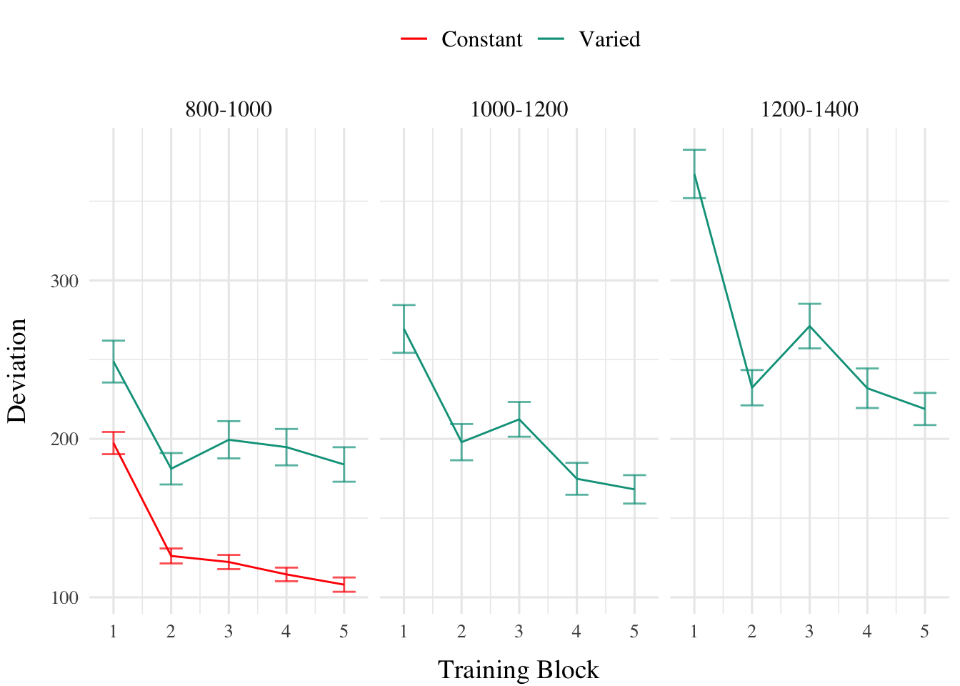
Figure 1: Experiment 1 Training Stage. Deviations from target band across training blocks. Lower values represent greater accuracy.
Table 1: Experiment 1 - End of training performance. The Intercept represents the average of the baseline (constant condition), and the conditVaried coefficient reflects the difference between the constant and varied groups. A larger positive estimates indicates a greater deviation (lower accuracy) for the varied group.
Term
Estimate
95% CrI Lower
95% CrI Upper
pd
Intercept
106.34
95.46
117.25
1
conditVaried
79.64
57.92
101.63
1
Training. Figure 1 displays the average deviations across training blocks for the varied group, which trained on three velocity bands, and the constant group, which trained on one velocity band. To compare the training conditions at the end of training, we analyzed performance on the 800-1000 velocity band, which both groups trained on. The full model results are shown in Table 1. The varied group had a significantly greater deviation than the constant group in the final training block, (\(\beta\) = 79.64, 95% CrI [57.92, 101.63]; pd = 100%).
Table 2: Experiment 1 testing accuracy. Main effects of condition and band type (training vs. extrapolation), and the interaction between the two factors. Larger coefficients indicate larger deviations from the baselines (Condition=constant & bandType=Trained) - and a positive interaction coefficient indicates disproporionate deviation for the varied condition on the extrapolation bands
Term
Estimate
95% CrI Lower
95% CrI Upper
pd
Intercept
152.55
70.63
229.85
1.0
conditVaried
39.00
-21.10
100.81
0.9
bandTypeExtrapolation
71.51
33.24
109.60
1.0
conditVaried:bandTypeExtrapolation
66.46
32.76
99.36
1.0
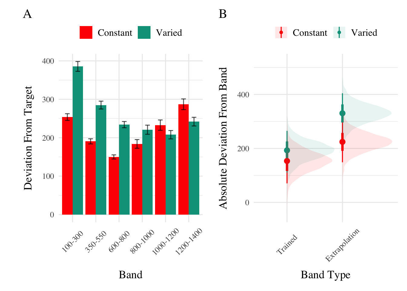
Testing. To compare accuracy between groups in the testing stage, we fit a Bayesian mixed effects model predicting deviation from the target band as a function of training condition (varied vs. constant) and band type (trained vs. extrapolation), with random intercepts for participants and bands. The model results are shown in Table 2. The main effect of training condition was not significant (\(\beta\) = 39, 95% CrI [-21.1, 100.81]; pd = 89.93%). The extrapolation testing items had a significantly greater deviation than the training bands (\(\beta\) = 71.51, 95% CrI [33.24, 109.6]; pd = 99.99%). Most importantly, the interaction between training condition and band type was significant (\(\beta\) = 66.46, 95% CrI [32.76, 99.36]; pd = 99.99%), As shown in Figure 2, the varied group had disproportionately larger deviations compared to the constant group in the extrapolation bands.
Code
pe1td<-testE1|>ggplot(aes(x =vb, y =dist,fill=condit))+stat_summary(geom ="bar", position=position_dodge(), fun =mean)+stat_summary(geom ="errorbar", position=position_dodge(.9), fun.data =mean_se, width =.4, alpha =.7)+theme(legend.title=element_blank(),axis.text.x =element_text(angle =45, hjust =0.5, vjust =0.5))+labs(x="Band", y="Deviation From Target")condEffects<-function(m,xvar){m|>ggplot(aes(x ={{xvar}}, y =.value, color =condit, fill =condit))+stat_dist_pointinterval()+stat_halfeye(alpha=.1, height=.5)+theme(legend.title=element_blank(),axis.text.x =element_text(angle =45, hjust =0.5, vjust =0.5))}pe1ce<-bmtd|>emmeans(~condit+bandType)|>gather_emmeans_draws()|>condEffects(bandType)+labs(y="Absolute Deviation From Band", x="Band Type")p2<-(pe1td+pe1ce)+plot_annotation(tag_levels='A')#ggsave(here::here("Assets/figs", "e1_test-dev.png"), p2, width=8, height=4, bg="white")p2
Figure 2: A) Deviations from target band during testing without feedback stage. B) Conditional effect of condition (Constant vs. Varied) and testing band type (training vs. extrapolation) on testing accuracy. Error bars represent 95% credible intervals.
Code
##| label: tbl-e1-bmm-vx##| tbl-cap: "Experiment 1. Bayesian Mixed Model Predicting Vx as a function of condition (Constant vs. Varied) and Velocity Band"e1_vxBMM<-brm(vx~condit*bandInt+(1+bandInt|id), data=test,file=paste0(here::here("data/model_cache", "e1_testVxBand_RF_5k")), iter=5000,chains=4,silent=0, control=list(adapt_delta=0.94, max_treedepth=13))#GetModelStats(e1_vxBMM) |> kable(booktabs = TRUE)cd1<-get_coef_details(e1_vxBMM, "conditVaried")sc1<-get_coef_details(e1_vxBMM, "bandInt")intCoef1<-get_coef_details(e1_vxBMM, "conditVaried:bandInt")
Table 3: Experiment 1. Bayesian Mixed Model Predicting velocity as a function of condition (Constant vs. Varied) and Velocity Band. Larger coefficients on Band represent greater sensitivity/discrimination.
Term
Estimate
95% CrI Lower
95% CrI Upper
pd
Intercept
408.55
327.00
490.61
1.00
conditVaried
164.05
45.50
278.85
1.00
Band
0.71
0.62
0.80
1.00
condit*Band
-0.14
-0.26
-0.01
0.98
Finally, to assess the ability of both conditions to discriminate between velocity bands, we fit a model predicting velocity as a function of training condition and velocity band, with random intercepts and random slopes for each participant. See Table 4 for the full model results. The estimated coefficient for training condition (\(\beta\) = 164.05, 95% CrI [45.5, 278.85], pd = 99.61%) suggests that the varied group tends to produce harder throws than the constant group, but is not in and of itself useful for assessing discrimination. Most relevant to the issue of discrimination is the coefficient on the Band predictor (\(\beta\) = 0.71 95% CrI [0.62, 0.8], pd = 100%). Although the median slope does fall underneath the ideal of value of 1, the fact that the 95% credible interval does not contain 0 provides strong evidence that participants exhibited some discrimination between bands. The estimate for the interaction between slope and condition (\(\beta\) = -0.14, 95% CrI [-0.26, -0.01], pd = 98.39%), suggests that the discrimination was somewhat modulated by training condition, with the varied participants showing less sensitivity between bands than the constant condition. This difference is depicted visually in Figure 3.
Figure 3: Empirical distribution of velocities producing in testing stage. Translucent bands with dash lines indicate the correct range for each velocity band.
Experiment 1. Conditional effect of training condition and Band. Ribbons indicate 95% HDI. The steepness of the lines serves as an indicator of how well participants discriminated between velocity bands.
E1 Summary
In Experiment 1, we investigated how variability in training influenced participants’ ability learn and extrapolate in a visuomotor task. Our findings that training with variable conditions rresulted in lower final training performance is consistent with much of the prior researchon the influence of training variability (Raviv et al., 2022; Soderstrom & Bjork, 2015), and is particularly unsurprising in the present work, given that the constant group received three times the amount of training on the velocity band common to the two conditions.
More importantly, the varied training group exhibited significantly larger deviations from the target velocity bands during the testing phase, particularly for the extrapolation bands that were not encountered by either condition during training.
References
Bürkner, P.-C. (2017). Brms: An R Package for Bayesian Multilevel Models Using Stan. Journal of Statistical Software, 80, 1–28. https://doi.org/10.18637/jss.v080.i01
Makowski, D., Ben-Shachar, M. S., & Lüdecke, D. (2019). bayestestR: Describing Effects and their Uncertainty, Existence and Significance within the Bayesian Framework. Journal of Open Source Software, 4(40), 1541. https://doi.org/10.21105/joss.01541
Raviv, L., Lupyan, G., & Green, S. C. (2022). How variability shapes learning and generalization. Trends in Cognitive Sciences, S1364661322000651. https://doi.org/10.1016/j.tics.2022.03.007
Soderstrom, N. C., & Bjork, R. A. (2015). Learning versus performance: An integrative review. Perspectives on Psychological Science, 10(2), 176–199. https://doi.org/10.1177/1745691615569000
Team, R. C. (2020). R: A Language and Environment for Statistical Computing. R: A Language and Environment for Statistical Computing.