Experiment 2

pacman::p_load(dplyr,purrr,tidyr,tibble,ggplot2,
  brms,tidybayes, rstanarm,emmeans,broom,bayestestR,
  stringr, here,conflicted, patchwork, knitr,kableExtra)
#options(brms.backend="cmdstanr",mc.cores=4)
options(dplyr.summarise.inform = FALSE)
walk(c("brms","dplyr","bayestestR"), conflict_prefer_all, quiet = TRUE)
walk(c("Display_Functions","org_functions"), ~ source(here::here(paste0("Functions/", .x, ".R"))))
e2 <- readRDS(here("data/e2_08-04-23.rds")) 
e2Sbjs <- e2 |> group_by(id,condit) |> summarise(n=n())
testE2 <- e2 |> filter(expMode2 == "Test")
nbins=5
trainE2 <-  e2 |> filter(expMode2=="Train") |> group_by(id,condit, vb) |> 
    mutate(Trial_Bin = cut( gt.train, breaks = seq(1, max(gt.train),length.out=nbins+1),include.lowest = TRUE, labels=FALSE)) 
trainE2_max <- trainE2 |> filter(Trial_Bin == nbins, bandInt==600)

# e2 |> group_by(condit, bandOrder) |> summarise(n_distinct(id))

Methods & Procedure

The task and procedure of Experiment 2 was identical to Experiment 1, with the exception that the training and testing bands were reversed (see Figure 1). The Varied group trained on bands 100-300, 350-550, 600-800, and the constant group trained on band 600-800. Both groups were tested from all six bands. A total of 110 participants completed the experiment (Varied: 55, Constant: 55).

Figure 1: Experiment 2 Design. Constant and Varied participants complete different training conditions. The training and testing bands are the reverse of Experiment 1.

Results

p1 <- trainE2 |> ggplot(aes(x = Trial_Bin, y = dist, color = condit)) +
    stat_summary(geom = "line", fun = mean) +
    stat_summary(geom = "errorbar", fun.data = mean_se, width = .4, alpha = .7) +
    facet_wrap(~vb)+
    scale_x_continuous(breaks = seq(1, nbins + 1)) +
    theme(legend.title=element_blank()) + 
    labs(y = "Deviation", x="Training Block") 
#ggsave(here("Assets/figs/e2_train_deviation.png"), p1, width = 8, height = 4,bg="white")
p1

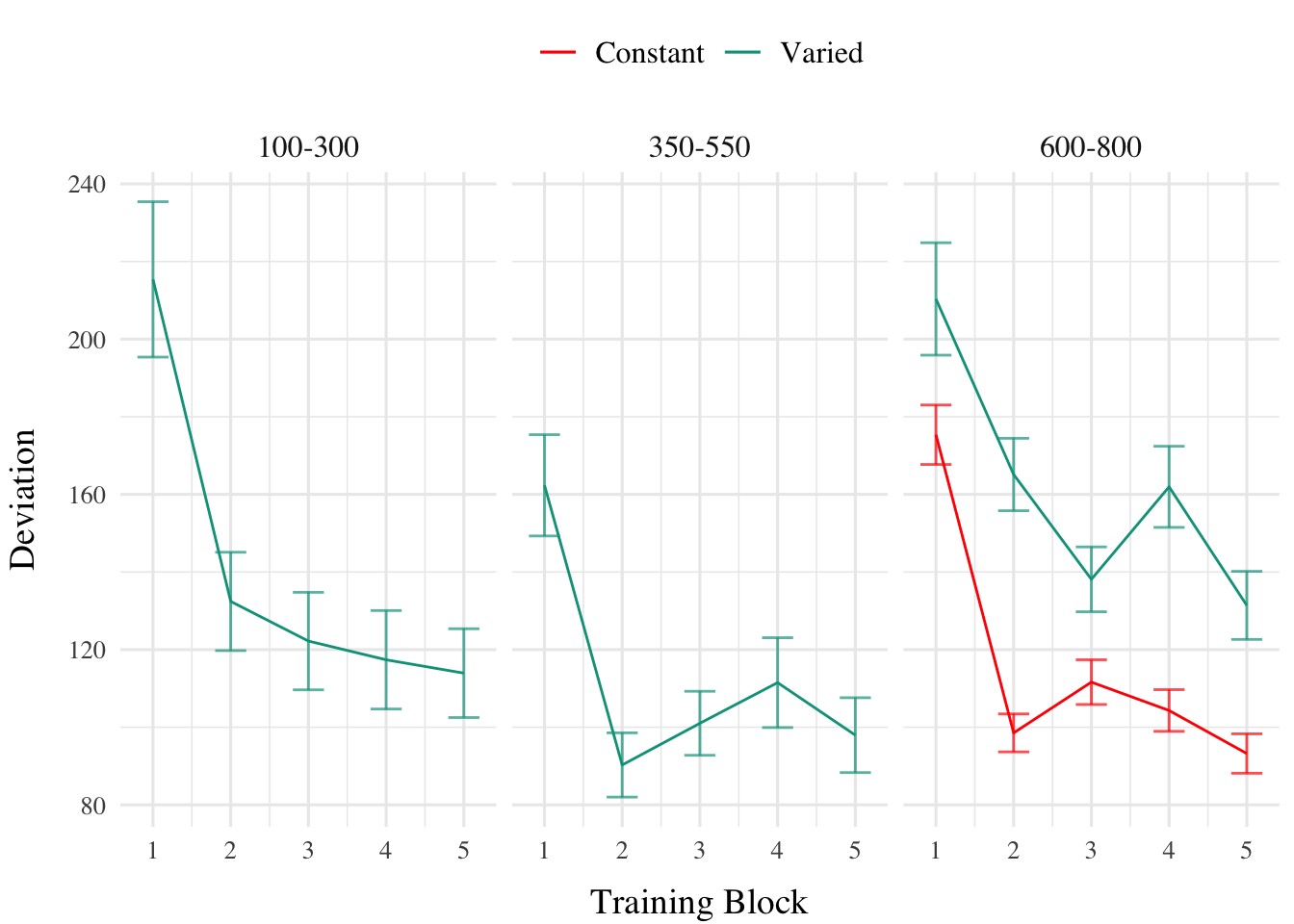
Figure 2: Experiment 2 Training Stage. Deviations from target band across training blocks. Lower values represent greater accuracy.

bmm_e2_train <- trainE2_max %>% 
  brm(dist ~ condit, 
      file=here("data/model_cache/e2_train_deviation"),
      data = .,
      iter = 2000,
      chains = 4,
      control = list(adapt_delta = .94, max_treedepth = 13))

mtr2 <- as.data.frame(describe_posterior(bmm_e2_train, centrality = "Mean"))[, c(1,2,4,5,6)]
colnames(mtr2) <- c("Term", "Estimate","95% CrI Lower", "95% CrI Upper", "pd")

cdtr2 <- get_coef_details(bmm_e2_train, "conditVaried")
# mtr2 |> mutate(across(where(is.numeric), \(x) round(x, 2))) |>
#   tibble::remove_rownames() |> 
#   mutate(Term = stringr::str_remove(Term, "b_")) |>
#   kable(escape=F,booktabs=T) 

Table 1: Experiment 2 - End of training performance. The Intercept represents the average of the baseline (constant condition), and the conditVaried coefficient reflects the difference between the constant and varied groups. A larger positive coefficient indicates a greater deviation (lower accuracy) for the varied group.

Term	Estimate	95% CrI Lower	95% CrI Upper	pd
Intercept	91.01	80.67	101.26	1
conditVaried	36.15	16.35	55.67	1

Training. Figure 2 presents the deviations across training blocks for both constant and varied training groups. We again compared training performance on the band common to both groups (600-800). The full model results are shown in Table 1. The varied group had a significantly greater deviation than the constant group in the final training block, ( \(\beta\) = 36.15, 95% CrI [16.35, 55.67]; pd = 99.95%).

modelFile <- paste0(here::here("data/model_cache/"), "e2_dist_Cond_Type_RF_2")
bmtd2 <- brm(dist ~ condit * bandType + (1|bandInt) + (1|id), 
    data=testE2, file=modelFile,
    iter=5000,chains=4, control = list(adapt_delta = .94, max_treedepth = 13))
                        
# mted2 <- as.data.frame(describe_posterior(bmtd2, centrality = "Mean"))[, c(1,2,4,5,6)]
# colnames(mted2) <- c("Term", "Estimate","95% CrI Lower", "95% CrI Upper", "pd")
# mted2 |> mutate(across(where(is.numeric), \(x) round(x, 2))) |>
#   tibble::remove_rownames() |> 
#   mutate(Term = stringr::str_remove(Term, "b_")) |>
#   kable(booktabs=TRUE) 

cd2ted1 <- get_coef_details(bmtd2, "conditVaried")
cd2ted2 <-get_coef_details(bmtd2, "bandTypeExtrapolation")
cd2ted3 <-get_coef_details(bmtd2, "conditVaried:bandTypeExtrapolation")

Table 2: Experiment 2 testing accuracy. Main effects of condition and band type (training vs. extrapolation), and the interaction between the two factors. Larger coefficient estimates indicate larger deviations from the baselines (constant & trained bands) - and a positive interaction coefficient indicates disproporionate deviation for the varied condition on the extrapolation bands

Term	Estimate	95% CrI Lower	95% CrI Upper	pd
Intercept	190.91	125.03	259.31	1.00
conditVaried	-20.58	-72.94	33.08	0.78
bandTypeExtrapolation	38.09	-6.94	83.63	0.95
conditVaried:bandTypeExtrapolation	82.00	41.89	121.31	1.00

 

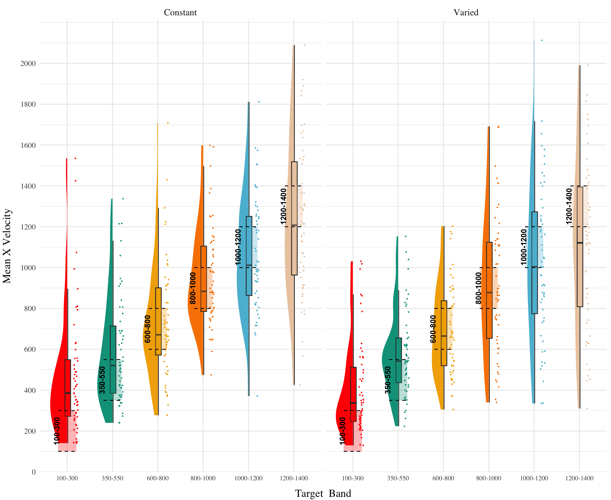
Testing Accuracy. The analysis of testing accuracy examined deviations from the target band as influenced by training condition (Varied vs. Constant) and band type (training vs. extrapolation bands). The results, summarized in Table 2, reveal no significant main effect of training condition (\(\beta\) = -20.58, 95% CrI [-72.94, 33.08]; pd = 77.81%). However, the interaction between training condition and band type was significant (\(\beta\) = 82, 95% CrI [41.89, 121.31]; pd = 100%), with the varied group showing disproportionately larger deviations compared to the constant group on the extrapolation bands (see Figure 3).

condEffects <- function(m,xvar){
  m |> ggplot(aes(x = {{xvar}}, y = .value, color = condit, fill = condit)) + 
  stat_dist_pointinterval() + 
  stat_halfeye(alpha=.1, height=.5) +
  theme(legend.title=element_blank(),axis.text.x = element_text(angle = 45, hjust = 0.5, vjust = 0.5)) 
  
}
pe2td <- testE2 |>  ggplot(aes(x = vb, y = dist,fill=condit)) +
    stat_summary(geom = "bar", position=position_dodge(), fun = mean) +
    stat_summary(geom = "errorbar", position=position_dodge(.9), fun.data = mean_se, width = .4, alpha = .7) + 
  theme(legend.title=element_blank(),axis.text.x = element_text(angle = 45, hjust = 0.5, vjust = 0.5)) +
  labs(x="Band", y="Deviation From Target")



pe2ce <- bmtd2 |> emmeans( ~condit + bandType) |>
  gather_emmeans_draws() |>
 condEffects(bandType) + labs(y="Absolute Deviation From Band", x="Band Type")

p2 <- (pe2td + pe2ce) + plot_annotation(tag_levels= 'A')
#ggsave(here::here("Assets/figs", "e2_test-dev.png"), p2, width=8, height=4, bg="white")
p2

Figure 3: A) Deviations from target band during testing without feedback stage. B) Estimated marginal means for the interaction between training condition and band type. Error bars represent 95% confidence intervals.

##| label: tbl-e2-bmm-vx
##| tbl-cap: "Experiment 2. Bayesian Mixed Model Predicting Vx as a function of condition (Constant vs. Varied) and Velocity Band"

e2_vxBMM <- brm(vx ~ condit * bandInt + (1 + bandInt|id),
                        data=test,file=paste0(here::here("data/model_cache", "e2_testVxBand_RF_5k")),
                        iter=5000,chains=4,silent=0,
                        control=list(adapt_delta=0.94, max_treedepth=13))

#GetModelStats(e2_vxBMM ) |> kable(escape=F,booktabs=T, caption="Fit to all 6 bands")

cd2 <- get_coef_details(e2_vxBMM, "conditVaried")
sc2 <- get_coef_details(e2_vxBMM, "bandInt")
intCoef2 <- get_coef_details(e2_vxBMM, "conditVaried:bandInt")

Table 3: Experiment 2. Bayesian Mixed Model Predicting Vx as a function of condition (Constant vs. Varied) and Velocity Band

Term	Estimate	95% CrI Lower	95% CrI Upper	pd
Intercept	362.64	274.85	450.02	1.00
conditVaried	-8.56	-133.97	113.98	0.55
Band	0.71	0.58	0.84	1.00
condit*Band	-0.06	-0.24	0.13	0.73

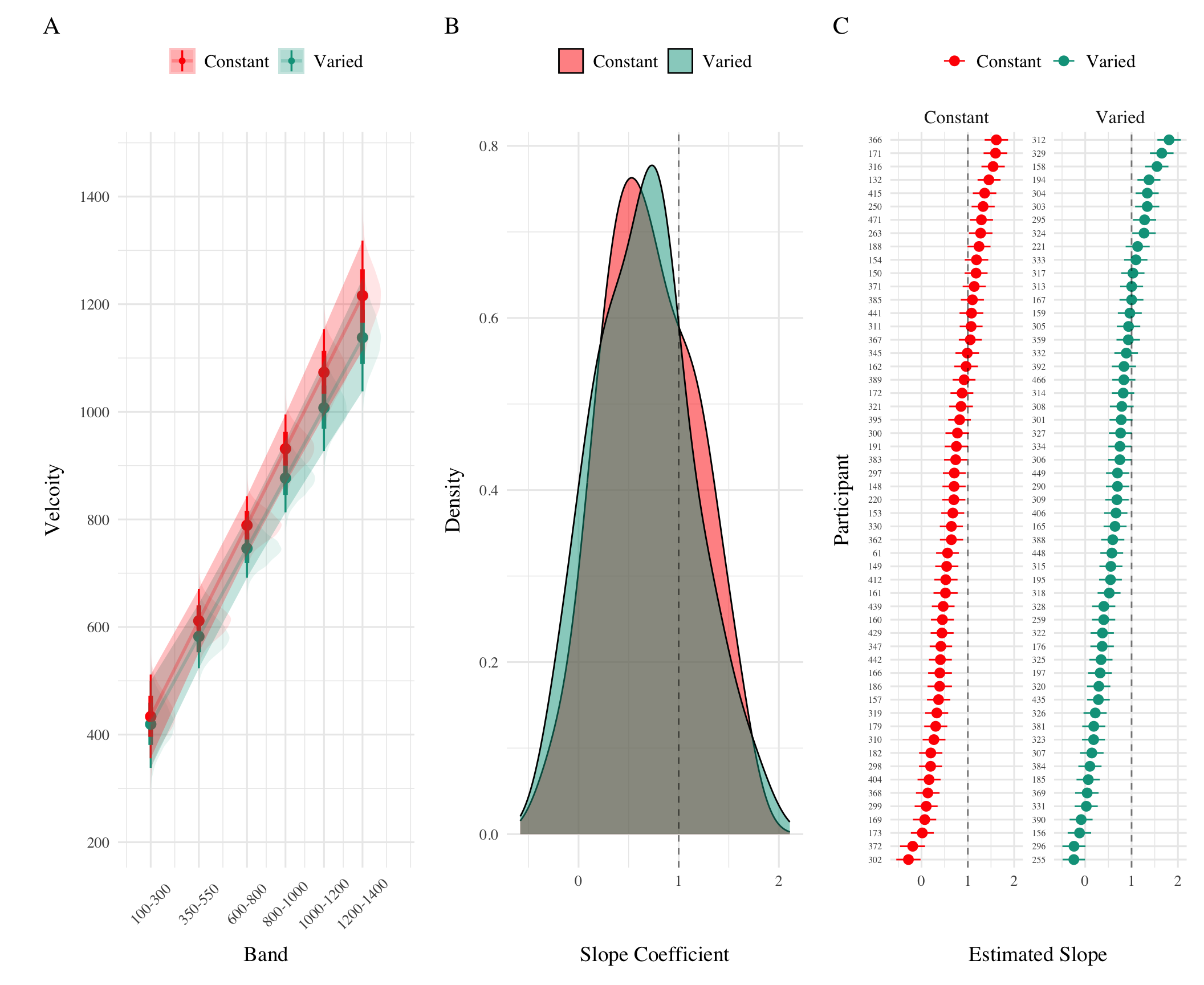
Testing Discrimination. Finally, to assess the ability of both conditions to discriminate between velocity bands, we fit a model predicting velocity as a function of training condition and velocity band, with random intercepts and random slopes for each participant. The full model results are shown in Table 4. The overall slope on target velocity band predictor was significantly positive, (\(\beta\) = 0.71, 95% CrI [0.58, 0.84]; pd= 100%), indicating that participants exhibited discrimination between bands. The interaction between slope and condition was not significant, (\(\beta\) = -0.06, 95% CrI [-0.24, 0.13]; pd= 72.67%), suggesting that the two conditions did not differ in their ability to discriminate between bands (see Figure 4).

testE2 %>% group_by(id,vb,condit) |> plot_distByCondit()

Figure 4: E2 testing x velocities. Translucent bands with dash lines indicate the correct range for each velocity band.

condEffects <- function(m,xvar){
  m |> ggplot(aes(x = {{xvar}}, y = .value, color = condit, fill = condit)) + 
  stat_dist_pointinterval() + 
  stat_halfeye(alpha=.1, height=.5) +
  theme(legend.title=element_blank(),axis.text.x = element_text(angle = 45, hjust = 0.5, vjust = 0.5)) 
}

pe2vce <- e2_vxBMM |> emmeans( ~condit + bandInt,re_formula=NA, 
                       at = list(bandInt = c(100, 350, 600, 800, 1000, 1200))) |>
  gather_emmeans_draws() |> 
  condEffects(bandInt) +
  stat_lineribbon(alpha = .25, size = 1, .width = c(.95)) +
  scale_x_continuous(breaks = c(100, 350, 600, 800, 1000, 1200), 
                     labels = levels(testE2$vb), 
                     limits = c(0, 1400)) + 
scale_y_continuous(expand=expansion(add=100),breaks=round(seq(0,2000,by=200),2)) +
  theme(legend.title=element_blank()) + 
  labs(y="Velcoity", x="Band")

fe <- fixef(e2_vxBMM)[,1]
fixed_effect_bandInt <- fixef(e2_vxBMM)[,1]["bandInt"]
fixed_effect_interaction <- fixef(e2_vxBMM)[,1]["conditVaried:bandInt"]

re <- data.frame(ranef(e2_vxBMM, pars = "bandInt")$id[, ,'bandInt']) |> 
  rownames_to_column("id") |> 
  left_join(e2Sbjs,by="id") |>
  mutate(adjust= fixed_effect_bandInt + fixed_effect_interaction*(condit=="Varied"),slope = Estimate + adjust )

pid_den2 <- ggplot(re, aes(x = slope, fill = condit)) + 
  geom_density(alpha=.5) + 
  geom_vline(xintercept = 1, linetype="dashed",alpha=.5) +
  xlim(c(min(re$slope)-.3, max(re$slope)+.3))+
   theme(legend.title=element_blank()) + 
  labs(x="Slope Coefficient",y="Density")

pid_slopes2 <- re |>  mutate(id=reorder(id,slope)) |>
  ggplot(aes(y=id, x=slope,fill=condit,color=condit)) + 
    geom_pointrange(aes(xmin=Q2.5+adjust, xmax=Q97.5+adjust)) + 
  geom_vline(xintercept = 1, linetype="dashed",alpha=.5) +
      theme(legend.title=element_blank(), 
        axis.text.y = element_text(size=6) ) + 
    labs(x="Estimated Slope", y="Participant")  + 
    ggh4x::facet_wrap2(~condit,axes="all",scales="free_y")

p3 <- (pe2vce + pid_den2 + pid_slopes2) + plot_annotation(tag_levels= 'A')
#ggsave(here::here("Assets/figs", "e2_test-vx.png"), p3,width=9,height=11, bg="white",dpi=600)
p3

Table 4

Conditional effect of training condition and Band. Ribbons indicate 95% HDI. The steepness of the lines serves as an indicator of how well participants discriminated between velocity bands.

Experiment 2 Summary

Experiment 2 extended the findings of Experiment 1 by examining the effects of training variability on extrapolation performance in a visuomotor function learning task, but with reversed training and testing bands. Similar to Experiment 1, the Varied group exhibited poorer performance during training and testing. However unlike experiment 1, the Varied group did not show a significant difference in discrimination between bands.