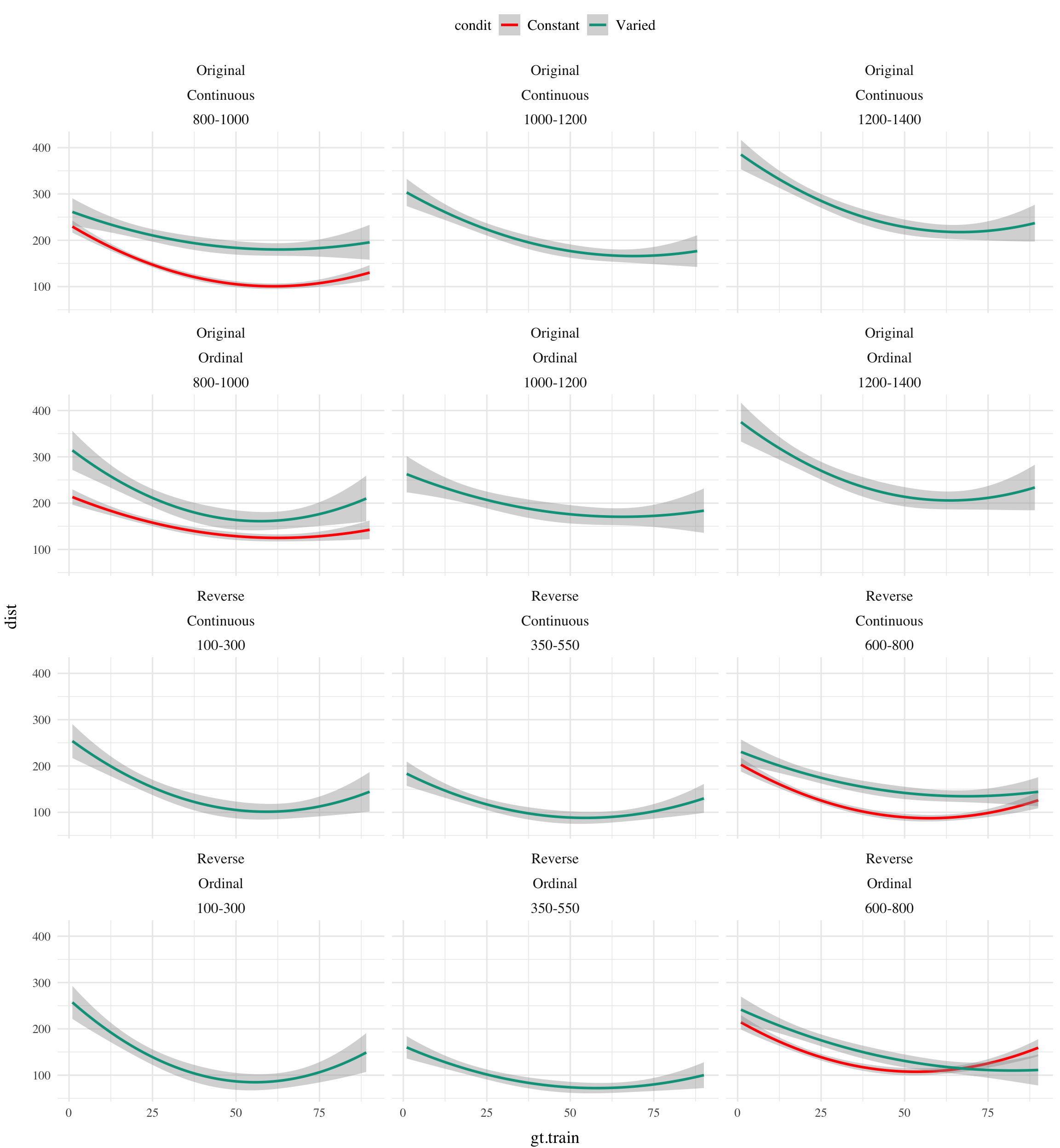
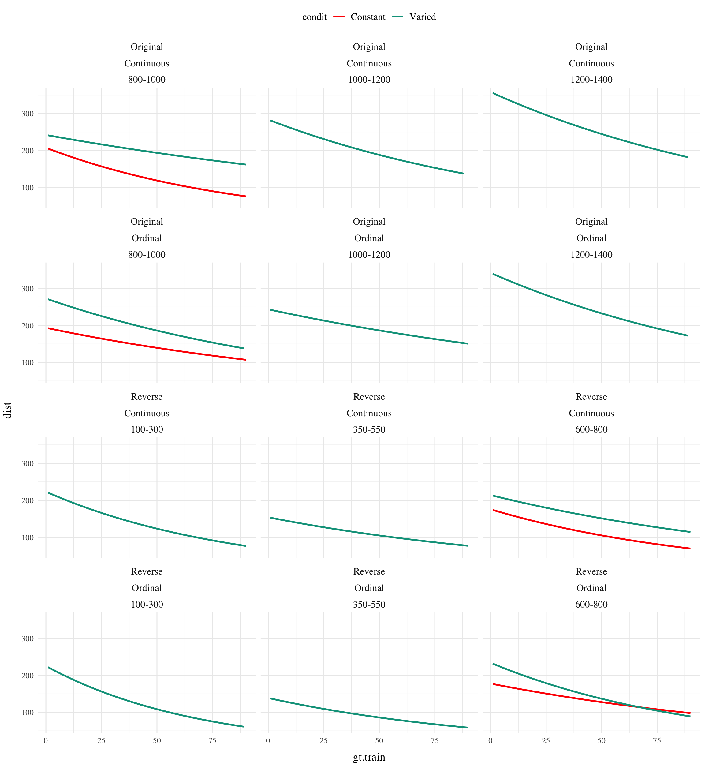
d|>filter(expMode=="train", gt.train<=60)|>group_by(id, gt.train, condit, vb)|>ggplot(aes(x =gt.train, y =dist, col =condit))+geom_smooth(method ="nls", formula =micmen.formula, se =FALSE, method.args =list(start =list(Vm =1, K =1)))+facet_wrap(~bandOrder*fb*vb, ncol =3)
Code
#bf(dist ~ betaMu + (alphaMu - betaMu) * exp(-exp(gammaMu) * gt.train)exp_model_formula<-y~a*exp(b*x)d|>filter(expMode=="train", gt.train<=60)%>%group_by(id, gt.train, condit, vb)%>%ggplot(aes(x =gt.train, y =dist, col =condit))+geom_smooth(method ="nls", formula =exp_model_formula, se =FALSE, method.args =list(start =list(a =1, b =0.1)))+facet_wrap(~bandOrder*fb*vb, ncol =3)
Warning: Removed 8188 rows containing non-finite outside the scale range
(`stat_smooth()`).
Code
three_param_exp_formula<-y~a+(b-a)*exp(-c*x)d|>filter(expMode=="train", gt.train<=60)%>%group_by(id, gt.train, condit, vb)%>%ggplot(aes(x =gt.train, y =dist, col =condit))+geom_smooth(method ="nls", formula =three_param_exp_formula, method.args =list(start =list(a =100, b =500, c =0.01)), # Starting values for a, b, c se =FALSE)+facet_wrap(~bandOrder*fb*vb, ncol =3)
Warning: Failed to fit group 1.
Caused by error in `method()`:
! singular gradient
Warning: Failed to fit group 2.
Caused by error in `method()`:
! singular gradient
Code
two_param_exp_formula<-y~a*exp(-c*x)d|>filter(expMode=="train")%>%group_by(id, gt.train, condit, vb)%>%ggplot(aes(x =gt.train, y =dist, col =condit))+geom_smooth(method ="nls", formula =two_param_exp_formula, method.args =list(start =list(a =500, c =0.09)), # Starting values for a, b, c se =FALSE)+facet_wrap(~bandOrder*fb*vb, ncol =3)
Code
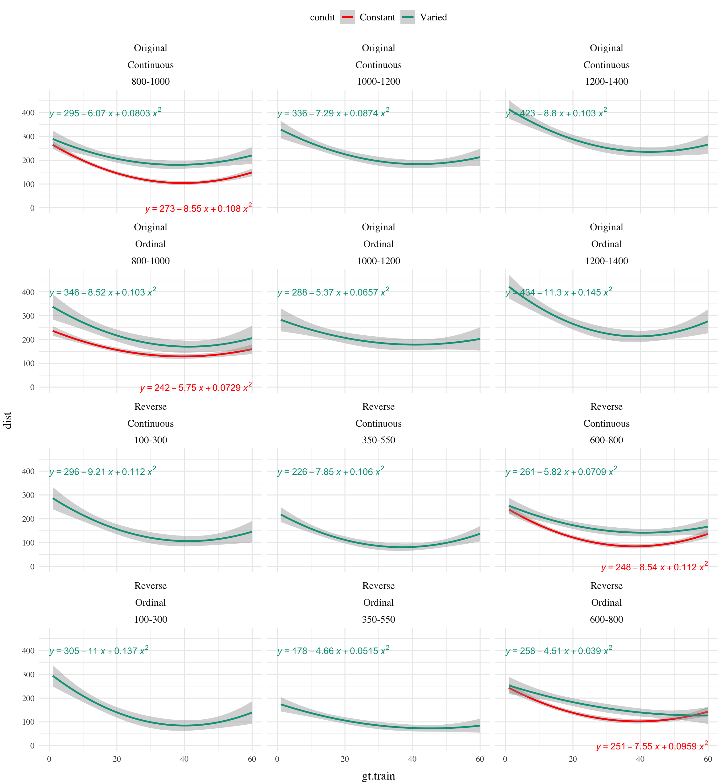
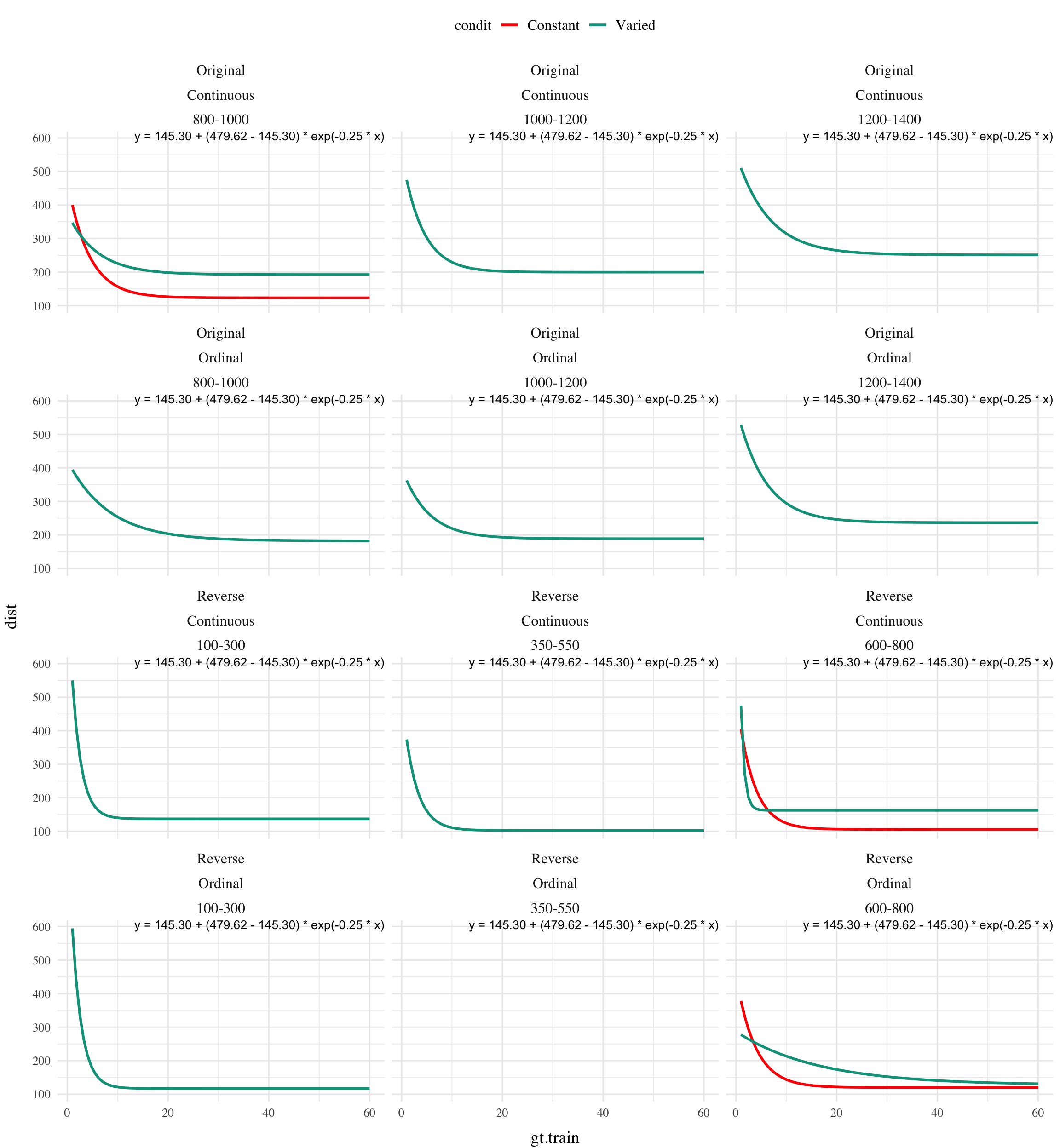
filtered_data<-d|>filter(expMode=="train", gt.train<=60)# Fit the modelnls_fit<-nls(dist~a+(b-a)*exp(-c*gt.train), data =filtered_data, start =list(a =100, b =500, c =0.01))# Extract coefficientscoeffs<-coef(nls_fit)# Create label (customize as needed)label_text<-sprintf("y = %.2f + (%.2f - %.2f) * exp(-%.2f * x)", coeffs["a"], coeffs["b"], coeffs["a"], coeffs["c"])# Plot with custom labelfiltered_data%>%ggplot(aes(x =gt.train, y =dist, col =condit))+geom_smooth(method ="nls", formula =y~a+(b-a)*exp(-c*x), method.args =list(start =list(a =100, b =500, c =0.01)), se =FALSE)+ggpp::annotate("text", x =Inf, y =Inf, label =label_text, hjust =1, vjust =1, size =3.5)+facet_wrap(~bandOrder*fb*vb, ncol =3)
Warning: Failed to fit group 1.
Caused by error in `method()`:
! singular gradient
Warning: Failed to fit group 2.
Caused by error in `method()`:
! singular gradient
Code
library(ggpmisc)d|>filter(expMode=="train", gt.train<=60)%>%group_by(id, gt.train, condit, vb)%>%ggplot(aes(x =gt.train, y =dist, col =condit))+geom_smooth(method ="nlsLM", formula =y~three_param_exp_formula(x, a, b, c), method.args =list(start =list(a =100, b =500, c =0.01)), se =FALSE)+# stat_equation(aes(label = after_stat(eq.label)),# formula = y ~ three_param_exp_formula(x, a, b, c),# parse = TRUE) +facet_wrap(~bandOrder*fb*vb, ncol =3)
Warning: Computation failed in `stat_smooth()`.
Caused by error in `get()`:
! object 'nlsLM' of mode 'function' was not found
Warning: Computation failed in `stat_smooth()`.
Computation failed in `stat_smooth()`.
Computation failed in `stat_smooth()`.
Computation failed in `stat_smooth()`.
Computation failed in `stat_smooth()`.
Computation failed in `stat_smooth()`.
Computation failed in `stat_smooth()`.
Computation failed in `stat_smooth()`.
Computation failed in `stat_smooth()`.
Computation failed in `stat_smooth()`.
Computation failed in `stat_smooth()`.
Caused by error in `get()`:
! object 'nlsLM' of mode 'function' was not found
Join the labels back to the original data
filtered_data <- left_join(filtered_data, labels_df, by = c(“condit”, “bandOrder”, “fb”))
Plot with annotations
ggplot(filtered_data, aes(x = gt.train, y = dist, col = condit)) + geom_smooth(method = “nls”, formula = y ~ a + (b - a) * exp(-c * x), method.args = list(start = list(a = 100, b = 500, c = 0.01)), se = FALSE) + facet_wrap(~bandOrder * fb * vb, ncol = 3) + geom_text(data = labels_df, aes(label = label, x = 50, y = Inf), hjust = 0.5, vjust = 1, size = 3, inherit.aes = FALSE)
Code
fit_model_and_return_label<-function(data, condit, bandOrder, fb){# Default starting parametersstart_params<-list(a =100, b =500, c =0.01)# Adjust starting parameters for the problematic conditionif(condit=="Constant"&&fb=="Ordinal"){start_params<-list(a =100, b =250, c =0.01)}tryCatch({model<-nls(dist~a+(b-a)*exp(-c*gt.train), data =data, start =start_params)coeffs<-coef(model)label=sprintf("y = %.2f + (%.2f - %.2f) * exp(-%.2f * x)", coeffs["a"], coeffs["b"], coeffs["a"], coeffs["c"])data.frame(label =label, a =coeffs["a"], b =coeffs["b"], c =coeffs["c"])}, error =function(e){# Return NA or some indication of failurereturn(data.frame(label =NA, a =NA, b =NA, c =NA))})}labels_df<-filtered_data%>%group_by(condit, bandOrder, fb,vb)%>%nest()%>%mutate(result =map(data, ~fit_model_and_return_label(.x, condit, bandOrder, fb)), data =NULL)%>%unnest(result)%>%ungroup()head(labels_df)
# A tibble: 6 × 8
condit fb vb bandOrder label a b c
<fct> <fct> <fct> <fct> <chr> <dbl> <dbl> <dbl>
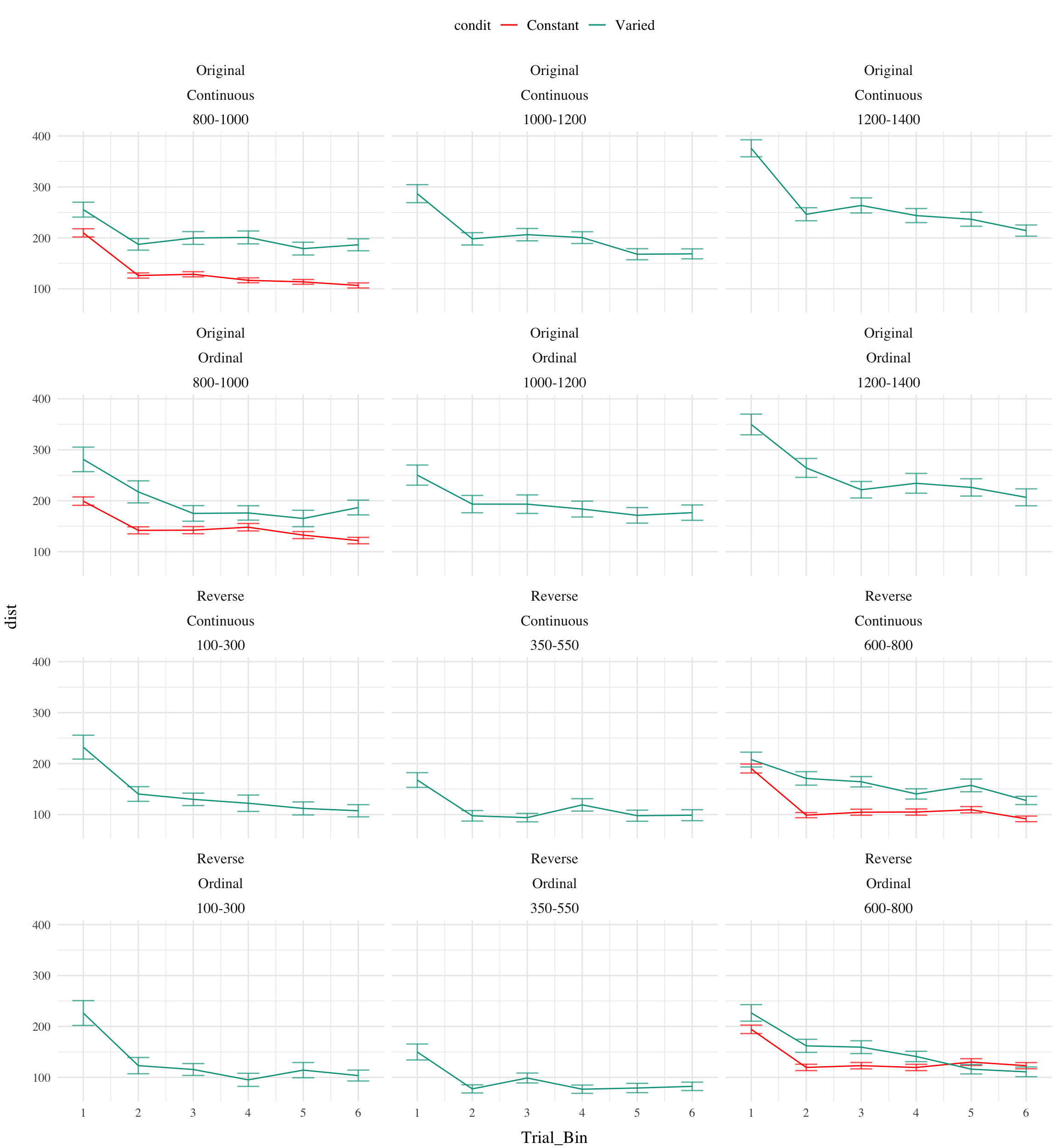
1 Varied Continuous 1000-1200 Original y = 199.90 + (551.8… 200. 552. 0.247
2 Varied Continuous 1200-1400 Original y = 251.42 + (553.9… 251. 554. 0.156
3 Varied Continuous 800-1000 Original y = 192.56 + (375.6… 193. 376. 0.171
4 Constant Continuous 800-1000 Original y = 123.33 + (473.5… 123. 474. 0.236
5 Constant Continuous 600-800 Reverse y = 105.74 + (513.6… 106. 514. 0.308
6 Varied Continuous 350-550 Reverse y = 102.66 + (502.0… 103. 502. 0.386
Code
generate_predictions<-function(x, a, b, c){return(a+(b-a)*exp(-c*x))}plot_data<-filtered_data%>%left_join(labels_df, by =c("condit", "bandOrder", "fb"))
Warning in left_join(., labels_df, by = c("condit", "bandOrder", "fb")): Detected an unexpected many-to-many relationship between `x` and `y`.
ℹ Row 1 of `x` matches multiple rows in `y`.
ℹ Row 1 of `y` matches multiple rows in `x`.
ℹ If a many-to-many relationship is expected, set `relationship =
  "many-to-many"` to silence this warning.
Code
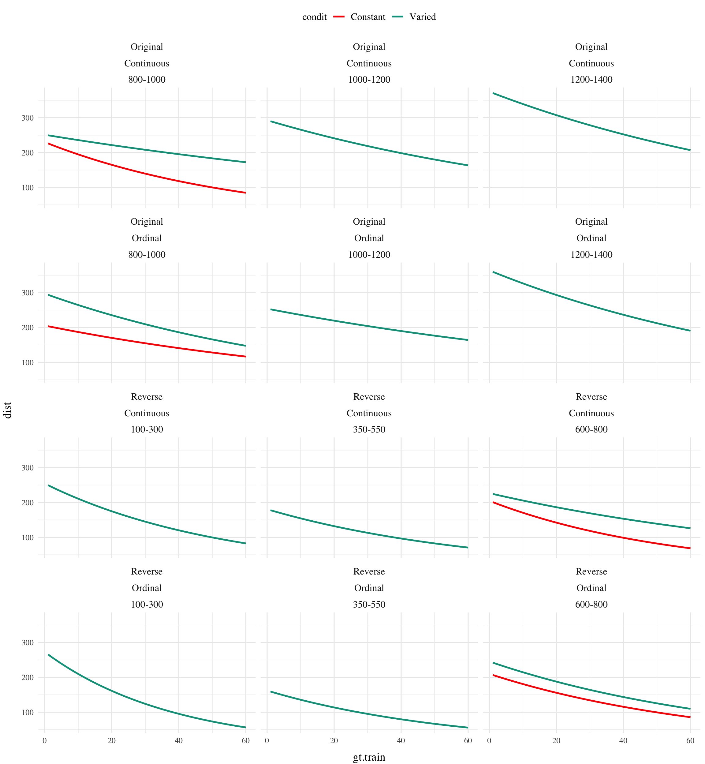
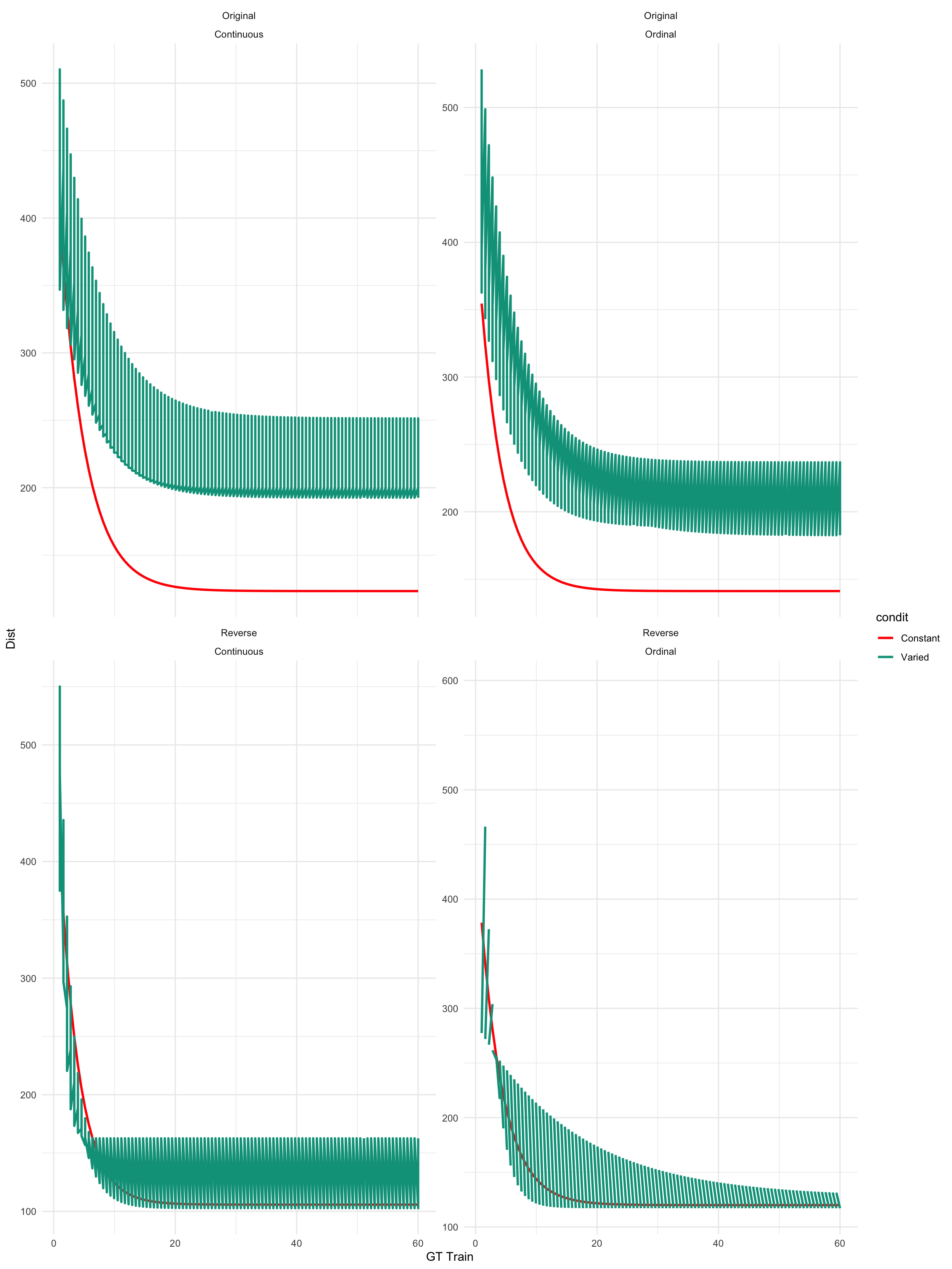
# Define a sequence of x values for generating model predictions (adjust as needed)x_vals<-seq(min(filtered_data$gt.train), max(filtered_data$gt.train), length.out =100)# Create a new data frame for model predictionspredictions_data<-labels_df%>%mutate(x =list(x_vals))%>%unnest(x)%>%mutate(y =pmap_dbl(list(a, b, c, x), ~generate_predictions(..4, ..1, ..2, ..3)))# Plotggplot()+#geom_point(data = plot_data, aes(x = gt.train, y = dist, color = condit), alpha = 0.6) +geom_line(data =predictions_data, aes(x =x, y =y, color =condit), size =1)+facet_wrap(~bandOrder*fb , ncol =2, scales ="free_y")+labs(x ="GT Train", y ="Dist")+theme_minimal()
Warning: Using `size` aesthetic for lines was deprecated in ggplot2 3.4.0.
ℹ Please use `linewidth` instead.
Code
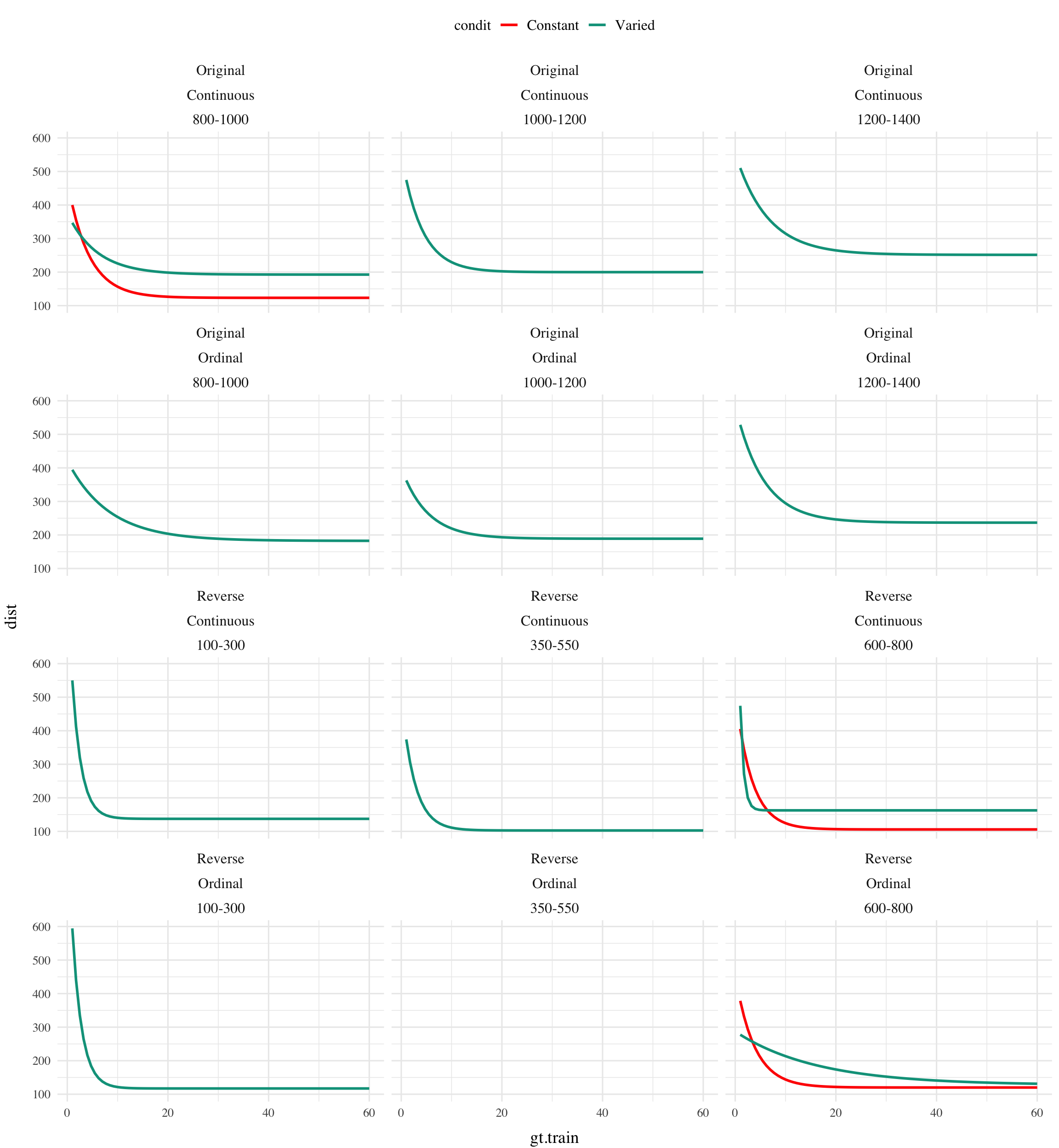
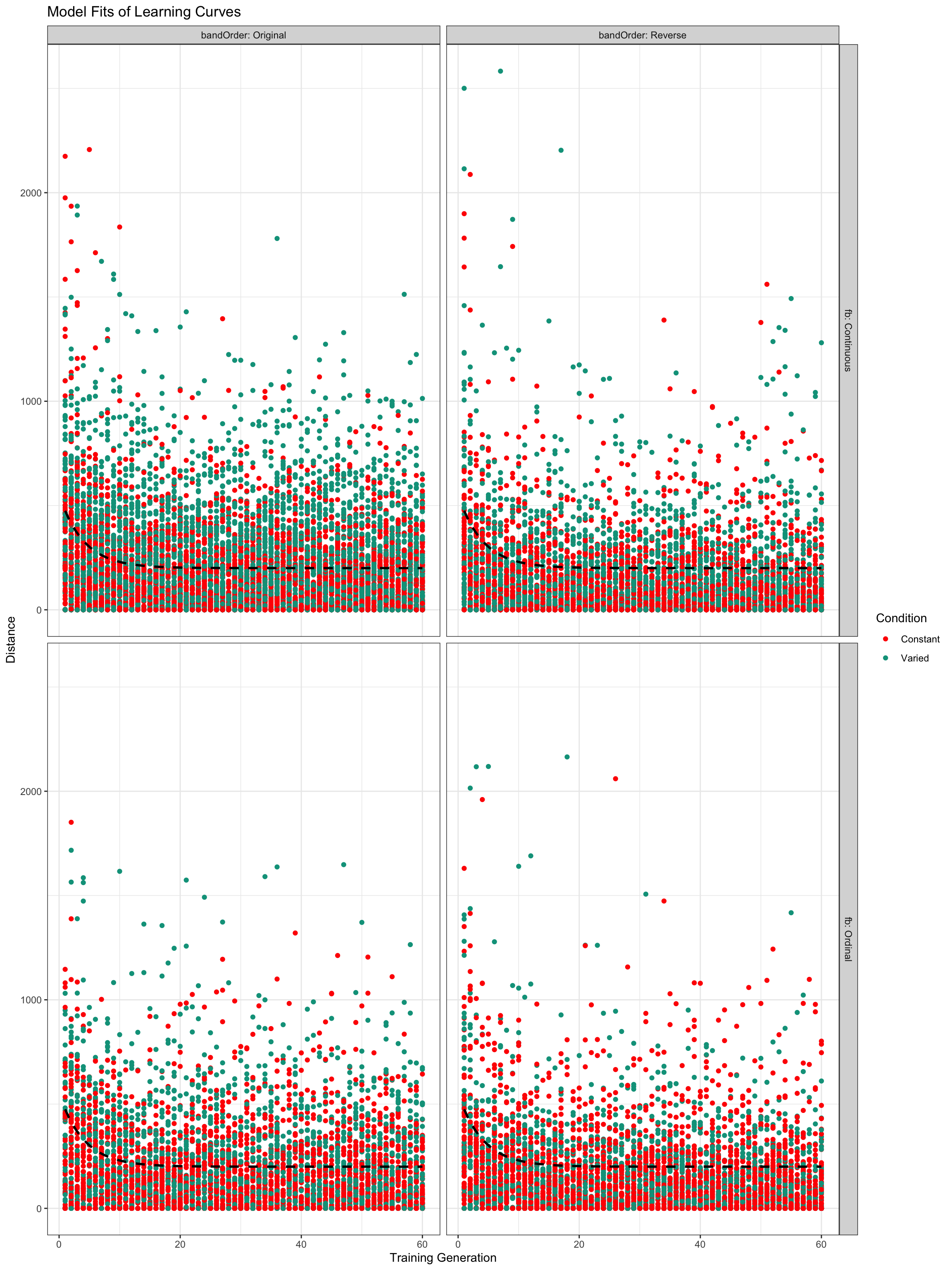
ggplot(filtered_data, aes(x =gt.train, y =dist, color =condit))+geom_point()+stat_function(fun =function(x)with(labels_df[1, ], a+(b-a)*exp(-c*x)), linetype ="dashed", color ="black", size =1)+facet_grid(fb~bandOrder, labeller =label_both)+labs(title ="Model Fits of Learning Curves", x ="Training Generation", y ="Distance", color ="Condition")+theme_bw()
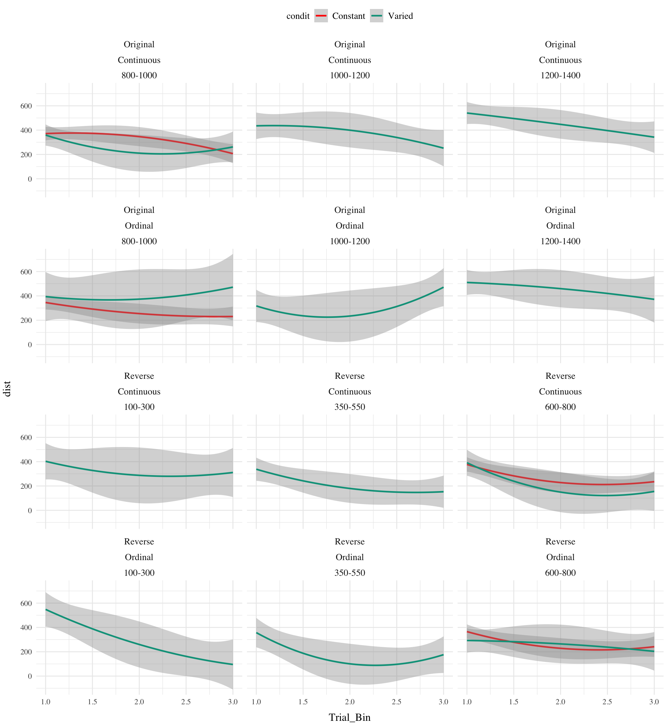
create learning models for condit and varied groups.
We can model the relation between performance and the number of practice trials as a power law function, or exponential function. Aggregatign over ids in dst. The models predict dist as an exponential decay function of trial number. Band is an additional predictor.
\[
f_p(t) = \alpha + \beta t^{r} \enspace
\]
\[
f_e(t) = \alpha + \beta e^{rt} \enspace
\]
Code
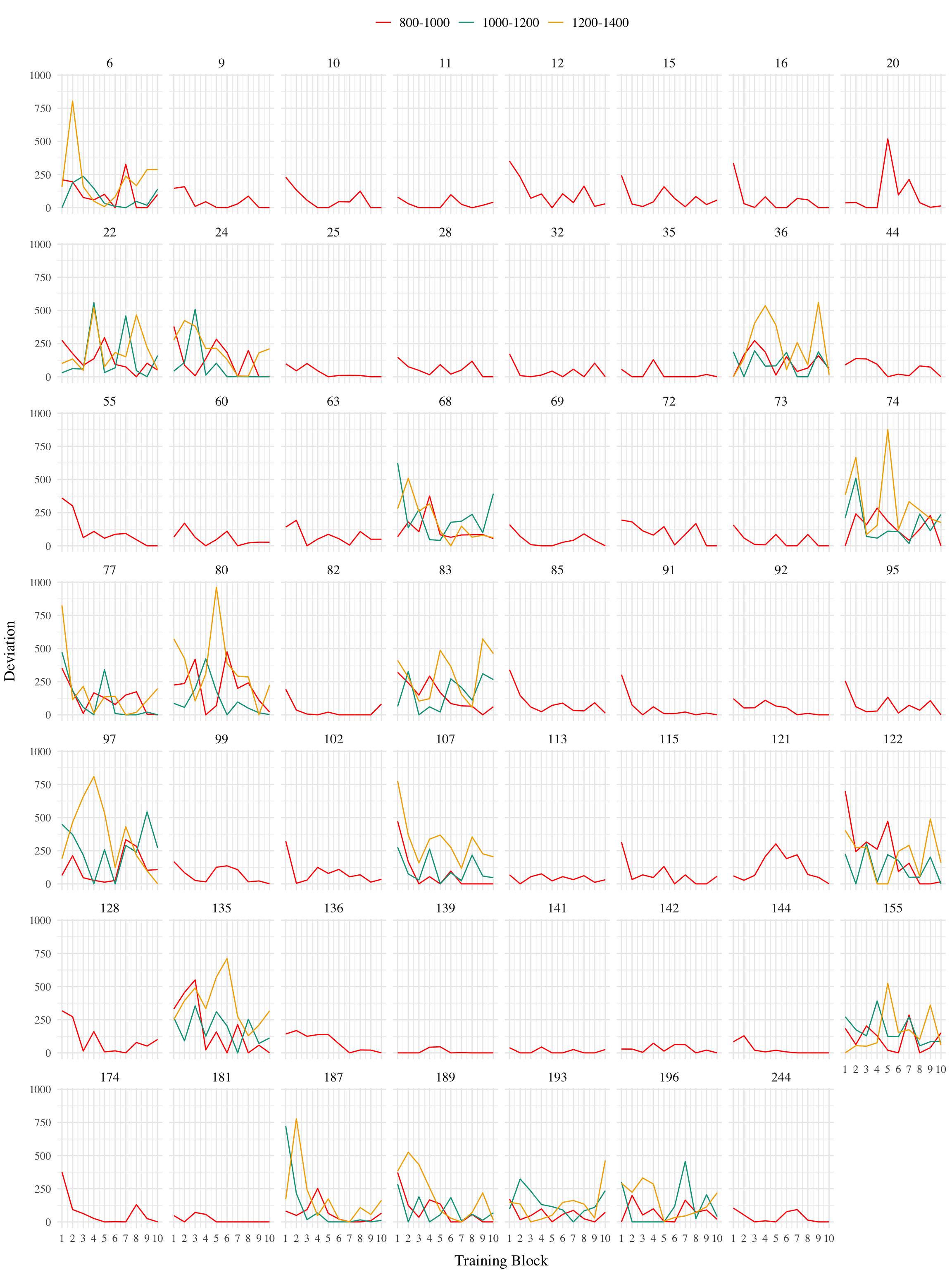
# fit exponential decay model as a function of trial numberfit_exp<-function(trial,dist,input){# fit exponential decay model as a function of trial number, band is an additional predictorfit<-nls(dist~yf+(y0-yf)*exp(-r*trial)+beta2*input, start =list(yf =300, y0 =364, beta2=0, r =.1), data =data.frame(trial=trial,dist=dist,input=input))# extract parametersalpha<-coef(fit)[1]beta<-coef(fit)[2]beta2<-coef(fit)[3]r<-coef(fit)[4]sigma_e<-summary(fit)$sigma# compute negative log likelihoodnllh<-negative_llh_exp(dist, trial, alpha, beta, r, sigma_e)# return parameters and negative log likelihoodreturn(list(alpha=alpha,beta=beta,beta2=beta2,r=r,sigma_e=sigma_e,nllh=nllh))}# Compute group averages for dist over trial and band. dst avgTrain<-e1|>filter(expMode2=="Train")%>%group_by(id,condit,gt.train,vb,bandInt)%>%summarise(dist=mean(dist))%>%ungroup()%>%group_by(condit,gt.train,vb,bandInt)%>%summarise(dist=mean(dist))%>%ungroup()ggplot(avgTrain,aes(x=gt.train,y=dist))+geom_line(aes(group=vb,color=vb))+facet_grid(~condit)avgTrain%>%filter(condit=="Constant")%>%nls(dist~yf+(y0-yf)*exp(-r*gt.train), start =list(yf =120, y0 =364, r =.1), data =.)%>%summary()avgTrain%>%filter(condit=="Constant")%>%nls(dist~SSasymp(gt.train, yf, y0, log_alpha),data=.)fit_condit<-avgTrain%>%group_by(condit)%>%do(fit_exp(trial=.$gt.train,dist=.$dist,input=.$bandInt))#avgTrain %>% group_by(condit) |> mutate(fit=map(~fit_exp(trial=gt.train,dist=dist,input=bandInt)))
Interpretation of improvement_model:
The intercept represents the performance when all factors are at their reference levels (Constant condition, original category order, and continuous feedback type). Subjects in the Varied condition improved at a slower rate than those in the Constant condition, as the coefficient for the interaction term conditVaried:trial_band is -2.37284, with a t-value of -6.940. Subjects in the Varied condition with reversed category order showed a greater decrease in performance, as the coefficient for the interaction term conditVaried:bandOrderrev is -43.67731, with a t-value of -2.323. Other significant factors and interactions include trial_band, bandOrderrev, trial_band:bandOrderrev, and trial_band:fbordinal. Interpretation of final_performance_model:
The intercept represents the final performance when all factors are at their reference levels (Constant condition, original category order, and continuous feedback type). Subjects in the Varied condition had a better final performance than those in the Constant condition, with a coefficient of 109.73 and a t-value of 4.362. The interaction between the Varied condition and reversed category order (conditVaried:bandOrderrev) had a negative impact on the final performance, with a coefficient of -92.75 and a t-value of -2.342. The interaction between the Varied condition and ordinal feedback type (conditVaried:fbordinal) also had a negative impact on the final performance, with a coefficient of -85.44 and a t-value of -2.079. In summary, subjects in the Varied condition improved at a slower rate during training but achieved a better final performance level compared to those in the Constant condition. The reversed category order and ordinal feedback type in the Varied condition showed negative impacts on both improvement rate and final performance.
Exponential learning model
Code
library(dplyr)library(tidyr)library(nls.multstart)exp_fun<-function(a, b, c, x){a*(1-exp(-b*x))+c}exp_models<-dst%>%nest(-id)%>%mutate(model =map(data, ~nls_multstart(dist~exp_fun(a, b, c, trial_band), data =.x, iter =500, start_lower =c(a =0, b =0, c =0), start_upper =c(a =5000, b =1, c =5000))))%>%unnest(c(a =map_dbl(model, ~coef(.x)['a']), b =map_dbl(model, ~coef(.x)['b']), c =map_dbl(model, ~coef(.x)['c'])))group_averages<-exp_models%>%group_by(condit, bandOrder, fb)%>%summarise(a_avg =mean(a), b_avg =mean(b), c_avg =mean(c))aic_improvement<-AIC(improvement_model)aic_final_performance<-AIC(final_performance_model)exp_models<-exp_models%>%mutate(aic =map_dbl(model, AIC))aic_exp_avg<-exp_models%>%summarise(aic_avg =mean(aic))