EXAM Group Fits

Simulation

ALM

EXAM

Published

March 27, 2024

Code

# load and view data
pacman::p_load(dplyr,purrr,tidyr,patchwork,here, pander, latex2exp, flextable)
purrr::walk(here::here(c("Functions/Display_Functions.R", "Functions/alm_core.R","Functions/fun_model.R")),source)
select <- dplyr::select; mutate <- dplyr::mutate 

ds <- readRDS(here::here("data/e1_md_11-06-23.rds"))
dsAvg <- ds |> group_by(condit,expMode2,tr, x) |> 
  summarise(y=mean(y),.groups="keep") 

vAvg <- dsAvg |> filter(condit=="Varied")
cAvg <- dsAvg |> filter(condit=="Constant")

#i1 <- ds |> filter(id=="3")

input.layer <- c(100,350,600,800,1000,1200)
output.layer <- c(100,350,600,800,1000,1200)


purrr::walk(c("con_group_exam_fits", "var_group_exam_fits", "hybrid_group_exam_fits"), 
            ~ list2env(readRDS(here::here(paste0("data/model_cache/", .x, ".rds"))), 
            envir = .GlobalEnv))

# pluck(ex_te_v, "Fit") |> mutate(w= ifelse(exists("w"), round(w,2),NA))
# pluck(hybrid_te_v, "Fit") |> mutate(w= ifelse(exists("w"), round(w,2), NA))

Code

 alm_plot()

Figure 1: The basic structure of the ALM model.

Table 1: ALM & EXAM Equations

	ALM Response Generation
Input Activation	$a_i(X) = \frac{e^{-c(X-X_i)^2}}{\sum_{k=1}^M e^{-c(X-X_k)^2}}$	Input nodes activate as a function of Gaussian similarity to stimulus
Output Activation	$O_j(X) = \sum_{k=1}^M w_{ji} \cdot a_i(X)$	Output unit $O_j$ activation is the weighted sum of input activations and association weights
Output Probability	$P[Y_j\|X] = \frac{O_j(X)}{\sum_{k=1}^M O_k(X)}$	The response, $Y_j$ probabilites computed via Luce’s choice rule
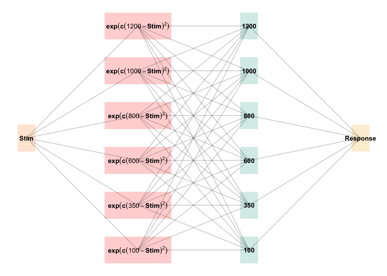
Mean Output	$m(X) = \sum_{j=1}^L Y_j \cdot \frac{O_j(x)}{\sum_{k=1}^M O_k(X)}$	Weighted average of probabilities determines response to X
	ALM Learning
Feedback	$f_j(Z) = e^{-c(Z-Y_j)^2}$	feedback signal Z computed as similarity between ideal response and observed response
magnitude of error	$\Delta_{ji}=(f_{j}(Z)-o_{j}(X))a_{i}(X)$	Delta rule to update weights.
Update Weights	$w_{ji}^{new}=w_{ji}+\eta\Delta_{ji}$	Updates scaled by learning rate parameter $\eta$.
	EXAM Extrapolation
Instance Retrieval	$P[X_i\|X] = \frac{a_i(X)}{\sum_{k=1}^M a_k(X)}$	Novel test stimulus $X$ activates input nodes $X_i$
Slope Computation	$S =$ $\frac{m(X_{1})-m(X_{2})}{X_{1}-X_{2}}$	Slope value, $S$ computed from nearest training instances
Response	$E[Y\|X_i] = m(X_i) + S \cdot [X - X_i]$	ALM response $m(X_i)$ adjusted by slope.

Modeling

In project 1, I applied model-based techniques to quantify and control for the similarity between training and testing experience, which in turn enabled us to account for the difference between varied and constant training via an extended version of a similarity based generalization model. In project 2, I will go a step further, implementing a full process model capable of both 1) producing novel responses and 2) modeling behavior in both the learning and testing stages of the experiment. For this purpose, we will apply the associative learning model (ALM) and the EXAM model of function learning (DeLosh 1997). ALM is a simple connectionist learning model which closely resembles Kruschke’s ALCOVE model (Kruscke 1992), with modifications to allow for the generation of continuous responses.

ALM & Exam Description

DeLosh et al. (1997) introduced the associative learning model (ALM), a connectionist model within the popular class of radial-basis networks. ALM was inspired by, and closely resembles Kruschke’s influential ALCOVE model of categorization (Kruschke, 1992).

ALM is a localist neural network model, with each input node corresponding to a particular stimulus, and each output node corresponding to a particular response value. The units in the input layer activate as a function of their Gaussian similarity to the input stimulus. So, for example, an input stimulus of value 55 would induce maximal activation of the input unit tuned to 55. Depending on thevalue of the generalization parameter, the nearby units (e.g. 54 and 56; 53 and 57) may also activate to some degree. ALM is structured with input and output nodes that correspond to regions of the stimulus space, and response space, respectively. The units in the input layer activate as a function of their similarity to a presented stimulus. As was the case with the exemplar-based models, similarity in ALM is exponentially decaying function of distance. The input layer is fully connected to the output layer, and the activation for any particular output node is simply the weighted sum of the connection weights between that node and the input activations. The network then produces a response by taking the weighted average of the output units (recall that each output unit has a value corresponding to a particular response). During training, the network receives feedback which activates each output unit as a function of its distance from the ideal level of activation necessary to produce the correct response. The connection weights between input and output units are then updated via the standard delta learning rule, where the magnitude of weight changes are controlled by a learning rate parameter.

See Table 1 for a full specification of the equations that define ALM and EXAM.

Model Fitting and Comparison

Following the procedure used by Mcdaniel et al. (2009), we will assess the ability of both ALM and EXAM to account for the empirical data when fitting the models to 1) only the training data, and 2) both training and testing data. Models were fit to the aggregated participant data by minimizing the root-mean squared deviation (RMSE). Because ALM has been shown to do poorly at accounting for human patterns extrapolation (DeLosh et al., 1997), we will also generate predictions from the EXAM model for the testing stage. EXAM which operates identically to ALM during training, but includes a linear extrapolation mechanism for generating novel responses during testing.

For the hybrid model, predictions are computed by first generating separate predictions from ALM and EXAM, and then combining them using the following equation: $\hat{y} = (1 - w) \cdot alm.pred + w \cdot exam.pred$. For the grid search, the weight parameter is varied from 0 to 1, and the resulting RMSE is recorded.

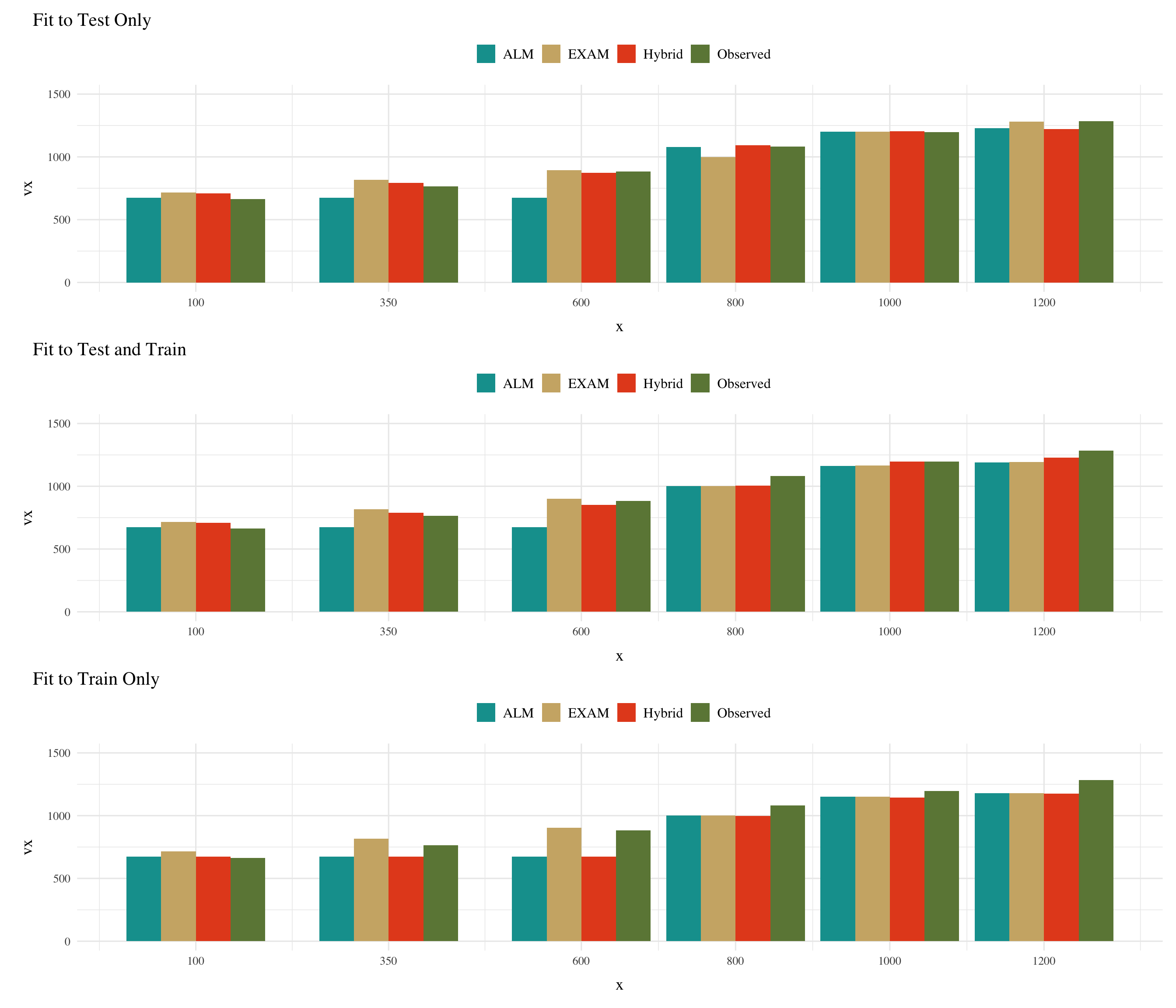
Each model was fit to the data in 3 different ways. 1) To just the testing data, 2) Both the training and testing data, 3) Only the training data. In all cases, the model only updates its weights during the training phase, and the weights are frozen during the testing phase. In all cases, only the ALM model generates predictions during the training phase. For the testing phase, all 3 models are used to generate predictions.

Code

##| column: body-outset-right


reshaped_df <- all_combined_params %>%
  select(-Value,-Test_RMSE) |>
  rename("Fit Method" = Fit_Method) |>
  pivot_longer(cols=c(c,lr,w),names_to="Parameter") %>%
  unite(Group, Group, Parameter) %>%
  pivot_wider(names_from = Group, values_from = value)

header_df <- data.frame(
  col_keys = c("Model", "Fit Method","Constant_c", "Constant_lr", "Constant_w", "Varied_c", "Varied_lr", "Varied_w"),
  line1 = c("", "", "Constant", "", "", "Varied", "",""),
  line2 = c("Model", "Fit Method", "c", "lr", "w", "c", "lr", "w")
)

ft <- flextable(reshaped_df) %>% 
  set_header_df(
    mapping = header_df,
    key = "col_keys"
  ) %>% add_header_lines(values = " ") %>%
  theme_booktabs() %>% 
  merge_v(part = "header") %>% 
  merge_h(part = "header") %>%
  merge_h(part = "header") %>%
  align(align = "center", part = "all") %>% 
  #autofit() %>% 
  empty_blanks() %>% 
  fix_border_issues() %>% 
  hline(part = "header", i = 2, j=3:5) %>% 
  hline(part = "header", i = 2, j=6:8)

ft

Table 2: Fit Parameters and Model RMSE. The Test_RMSE column is the main performance indicator of interest, and represents the RMSE for just the testing data. The Fit_Method column indicates the data used to fit the model. The $w$ parameter determines the balance between the ALM and EXAM response generation processes, and is only included for the hybrid model. A weight of .5 would indicate equal contribution from both models. $w$ values approaching 1 indicate stronger weight for EXAM.


		Constant			Varied
Model	Fit Method	c	lr	w	c	lr	w
ALM	Test Only	0.000	0.100		0.134	2.030
ALM	Test & Train	0.047	0.080		0.067	0.100
ALM	Train Only	0.060	0.100		0.047	0.080
EXAM	Test Only	0.007	1.327		0.409	1.910
EXAM	Test & Train	0.081	0.161		0.074	0.100
EXAM	Train Only	0.060	0.100		0.047	0.080
Hybrid	Test Only	0.008	1.580	1	0.395	2.017	0.64
Hybrid	Test & Train	0.067	0.134	1	0.134	2.017	0.79
Hybrid	Train Only	0.042	0.067	0	0.042	0.067	0.00

Testing Observations vs. Predictions

Code

tvte<- pluck(a_te_v, "test") |> 
  mutate(Fit_Method="Test Only") |>
  rename(ALM=pred,Observed=y) %>% 
  cbind(.,EXAM=pluck(ex_te_v, "test") |> pull(pred)) %>%
  cbind(., Hybrid=pluck(hybrid_te_v, "test") |> pull(pred))

tvtetr<-pluck(a_tetr_v, "test") |> 
  mutate(Fit_Method="Test & Train") |> 
  rename(ALM=pred,Observed=y) %>% 
  cbind(.,EXAM=pluck(ex_tetr_v, "test") |> pull(pred)) %>%
  cbind(., Hybrid=pluck(hybrid_tetr_v, "test") |> pull(pred))

tvtr<- pluck(a_tr_v, "test")|> 
  mutate(Fit_Method="Train Only") |> 
  rename(ALM=pred,Observed=y) %>% 
  cbind(.,EXAM=pluck(ex_tr_v, "test") |> pull(pred)) %>%
  cbind(., Hybrid=pluck(hybrid_tr_v, "test") |> pull(pred))

tcte<- pluck(a_te_c, "test") |> 
  mutate(Fit_Method="Test Only") |> 
  rename(ALM=pred,Observed=y) %>% 
  cbind(.,EXAM=pluck(ex0_te_c, "test") |> pull(pred)) %>%
  cbind(., Hybrid=pluck(hybrid_te_c, "test") |> pull(pred))

tctetr<-pluck(a_tetr_c, "test") |> 
  mutate(Fit_Method="Test & Train") |>  
  rename(ALM=pred,Observed=y) %>% 
  cbind(.,EXAM=pluck(ex0_tetr_c, "test") |> pull(pred)) %>%
  cbind(., Hybrid=pluck(hybrid_tetr_c, "test") |> pull(pred))

tctr<- pluck(a_tr_c, "test")|> 
  mutate(Fit_Method="Train Only") |>  
  rename(ALM=pred,Observed=y) %>% 
  cbind(.,EXAM=pluck(ex0_tr_c, "test") |> pull(pred)) %>%
  cbind(., Hybrid=pluck(hybrid_tr_c, "test") |> pull(pred))

vPreds <- rbind(tvte,tvtetr, tvtr) |> relocate(Fit_Method,.before=x) |> 
   mutate(across(where(is.numeric), \(x) round(x, 0)))

cPreds <- rbind(tcte,tctetr, tctr) |> relocate(Fit_Method,.before=x) |> 
   mutate(across(where(is.numeric), \(x) round(x, 0)))

allPreds <- rbind(vPreds |> mutate(Group="Varied"), cPreds |> mutate(Group="Constant")) |>
  pivot_longer(cols=c("ALM","EXAM","Hybrid"), names_to="Model",values_to = "Prediction") |> 
  mutate(Error=Observed-Prediction, Abs_Error=((Error)^2)) |> 
  group_by(Group,Fit_Method, Model) #|> summarise(Mean_Error=mean(Error), Abs_Error=mean(Abs_Error))

Code

allPreds |> summarise(Error=mean(Error), Abs_Error=sqrt(mean(Abs_Error))) |> 
  mutate(Fit_Method=factor(Fit_Method, levels=c("Test Only", "Test & Train", "Train Only"))) |>
  tabulator(rows=c("Fit_Method", "Model"), columns=c("Group"), 
             `ME` = as_paragraph(Error), 
            `RMSE` = as_paragraph(Abs_Error)) |> as_flextable()

Table 3: Model Perforamnce - averaged over all X values/Bands. ME=Mean Average Error, RMSE = Root mean squared error.

Fit_Method	Model	Constant		Varied
Fit_Method	Model	ME	RMSE	ME	RMSE
Test Only	ALM	223.8	348.0	56.3	95.4
	EXAM	-59.2	127.5	-6.0	45.9
	Hybrid	-58.2	127.4	-3.0	33.8
Test & Train	ALM	193.2	328.7	82.3	106.6
	EXAM	-28.8	132.1	13.2	60.2
	Hybrid	-16.7	136.7	16.7	46.5
Train Only	ALM	194.5	329.2	86.3	109.1
	EXAM	75.3	199.9	17.5	65.4
	Hybrid	197.5	330.4	88.3	110.3

Varied Testing Predictions

Code

##| column: screen-inset-right

####

vte <-  pluck(a_te_v, "test") |> rename(ALM=pred,Observed=y) %>% 
  cbind(.,EXAM=pluck(ex_te_v, "test") |> pull(pred)) %>%
  cbind(., Hybrid=pluck(hybrid_te_v, "test") |> pull(pred)) |>  
  pivot_longer(Observed:Hybrid, names_to="Model", values_to = "vx") |> 
  ggplot(aes(x,vx,fill=Model, group=Model)) +geom_bar(position="dodge",stat="identity") +
  scale_fill_manual(values=col_themes$wes2)+
  scale_x_continuous(breaks=sort(unique(ds$x)), labels=sort(unique(ds$x)))+ylim(0,1500) +
  theme(legend.title = element_blank(), legend.position="top") +ggtitle("Fit to Test Only")

vtetr <-  pluck(a_tetr_v, "test") |> rename(ALM=pred,Observed=y) %>% 
  cbind(.,EXAM=pluck(ex_tetr_v, "test") |> pull(pred)) %>%
  cbind(., Hybrid=pluck(hybrid_tetr_v, "test") |> pull(pred)) |>  
  pivot_longer(Observed:Hybrid, names_to="Model", values_to = "vx") |> 
  ggplot(aes(x,vx,fill=Model, group=Model)) +geom_bar(position="dodge",stat="identity") + 
  scale_fill_manual(values=col_themes$wes2)+
  scale_x_continuous(breaks=sort(unique(ds$x)), labels=sort(unique(ds$x)))+ylim(0,1500) +
  theme(legend.title = element_blank(), legend.position="top") +ggtitle("Fit to Test and Train")

vtr <-  pluck(a_tr_v, "test") |> rename(ALM=pred,Observed=y) %>% 
  cbind(.,EXAM=pluck(ex_tr_v, "test") |> pull(pred)) %>%
  cbind(., Hybrid=pluck(hybrid_tr_v, "test") |> pull(pred)) |>  
  pivot_longer(Observed:Hybrid, names_to="Model", values_to = "vx") |> 
  ggplot(aes(x,vx,fill=Model, group=Model)) +geom_bar(position="dodge",stat="identity") +
  scale_fill_manual(values=col_themes$wes2)+
  scale_x_continuous(breaks=sort(unique(ds$x)), labels=sort(unique(ds$x)))+ylim(0,1500) +
  theme(legend.title = element_blank(), legend.position="top") +ggtitle("Fit to Train Only")

 vte/vtetr/vtr

Figure 2: Varied Group - Mean Model predictions vs. observations

Code

##| column: screen-inset-right


# Create a custom header dataframe
header_df <- data.frame(
  col_keys = c("Fit_Method", "x","Observed" ,"ALM_Predicted", "ALM_Residual", "EXAM_Predicted","EXAM_Residual", "Hybrid_Predicted","Hybrid_Residual"),
  line1 = c("","","", "ALM", "", "EXAM", "", "Hybrid",""),
  line2 = c("Fit Method", "X", "Observed", "Predicted","Residual", "Predicted","Residual", "Predicted","Residual")
)


best_vPreds <- vPreds %>%
  pivot_longer(cols = c(ALM, EXAM, Hybrid), names_to = "Model", values_to = "Predicted") |>
  mutate(Residual=(Observed-Predicted), abs_res =abs(Residual)) |> group_by(Fit_Method,x) |>
  mutate(best=if_else(abs_res==min(abs_res),1,0)) |> select(-abs_res)

long_vPreds <- best_vPreds |> select(-best) |>
  pivot_longer(cols=c(Predicted,Residual), names_to="Model_Perf") |>
  relocate(Model, .after=Fit_Method) |> 
  unite(Model,Model,Model_Perf) |>
  pivot_wider(names_from=Model,values_from=value)

best_wide <- best_vPreds |> select(-Residual,-Predicted,-Observed) |> ungroup() |>
  pivot_wider(names_from=Model,values_from=best) |> select(ALM,EXAM,Hybrid)

best_indexV <- row_indices <- apply(best_wide, 1, function(row) {
 which(row == 1)
})


apply_best_formatting <- function(ft, best_index) {
  for (i in 1:length(best_index)) {
      #ft <- ft %>% surround(i=i,j=best_index[i],border=fp_border_default(color="red",width=1))
      ind = best_index[[i]]
      ind <- ind  %>% map_dbl(~ .x*2+3)
      ft <- ft %>% highlight(i=i,j=ind,color="wheat")
      }
  return(ft)
}

ft <- flextable(long_vPreds) %>% 
  set_header_df(
    mapping = header_df,
    key = "col_keys"
  ) %>% 
  theme_booktabs() %>% 
  merge_v(part = "header") %>% 
  merge_h(part = "header") %>%
  align(align = "center", part = "all") %>% 
  #autofit() %>% 
  empty_blanks() %>% 
  fix_border_issues() %>%
  hline(part = "header", i = 1, j=4:9) %>%
  vline(j=c("Observed","ALM_Residual","EXAM_Residual")) %>%
  hline(part = "body", i=c(6,12)) |> 
  bold(i=long_vPreds$x %in% c(100,350,600), j=2) 

  # bold the cell with the lowest residual, based on best_wide df
  # for each row, the cell that should be bolded matches which column in best_wide==1 at that row
ft <- apply_best_formatting(ft, best_indexV)
ft

Table 4: Varied group - mean model predictions vs. observations. Extrapolation Bands are bolded. For each Modelling fitting and band combination, the model with the smallest residual is highlighted. Only the lower bound of each velocity band is shown (bands are all 200 units).

			ALM		EXAM		Hybrid
Fit Method	X	Observed	Predicted	Residual	Predicted	Residual	Predicted	Residual
Test Only	100	663	675	-12	716	-53	708	-45
Test Only	350	764	675	89	817	-53	792	-28
Test Only	600	884	675	209	895	-11	875	9
Test Only	800	1,083	1,078	5	1,000	83	1,091	-8
Test Only	1,000	1,196	1,202	-6	1,199	-3	1,204	-8
Test Only	1,200	1,283	1,230	53	1,282	1	1,221	62
Test & Train	100	663	675	-12	716	-53	707	-44
Test & Train	350	764	675	89	817	-53	788	-24
Test & Train	600	884	675	209	902	-18	851	33
Test & Train	800	1,083	1,000	83	1,000	83	1,004	79
Test & Train	1,000	1,196	1,163	33	1,165	31	1,196	0
Test & Train	1,200	1,283	1,191	92	1,194	89	1,227	56
Train Only	100	663	675	-12	716	-53	675	-12
Train Only	350	764	675	89	817	-53	675	89
Train Only	600	884	675	209	905	-21	675	209
Train Only	800	1,083	1,000	83	1,000	83	999	84
Train Only	1,000	1,196	1,150	46	1,150	46	1,143	53
Train Only	1,200	1,283	1,180	103	1,180	103	1,176	107

Code

pander(tvte, caption="Varied fit to test only")
pander(tvtetr,caption="Varied fit to train and test")
pander(tvtr,caption="Varied fit to train only")

Constant Testing Predictions

Code

##| column: screen-inset-right

####

cte <-  pluck(a_te_c, "test") |> rename(ALM=pred,Observed=y) %>% 
  cbind(.,EXAM=pluck(ex0_te_c, "test") |> pull(pred)) %>%
  cbind(., Hybrid=pluck(hybrid_te_c, "test") |> pull(pred)) |>  
  pivot_longer(Observed:Hybrid, names_to="Model", values_to = "vx") |> 
  ggplot(aes(x,vx,fill=Model, group=Model)) +geom_bar(position="dodge",stat="identity") +
  scale_fill_manual(values=col_themes$wes2)+
  scale_x_continuous(breaks=sort(unique(ds$x)), labels=sort(unique(ds$x)))+ylim(0,1500) +
  theme(legend.title = element_blank(), legend.position="top") +ggtitle("Fit to Test Only")

ctetr <-  pluck(a_tetr_c, "test") |> rename(ALM=pred,Observed=y) %>% 
  cbind(.,EXAM=pluck(ex0_tetr_c, "test") |> pull(pred)) %>%
  cbind(., Hybrid=pluck(hybrid_tetr_c, "test") |> pull(pred)) |>  
  pivot_longer(Observed:Hybrid, names_to="Model", values_to = "vx") |> 
  ggplot(aes(x,vx,fill=Model, group=Model)) +geom_bar(position="dodge",stat="identity") + 
  scale_fill_manual(values=col_themes$wes2)+
  scale_x_continuous(breaks=sort(unique(ds$x)), labels=sort(unique(ds$x)))+ylim(0,1500) +
  theme(legend.title = element_blank(), legend.position="top") +ggtitle("Fit to Test and Train")

ctr <-  pluck(a_tr_c, "test") |> rename(ALM=pred,Observed=y) %>% 
  cbind(.,EXAM=pluck(ex0_tr_c, "test") |> pull(pred)) %>%
  cbind(., Hybrid=pluck(hybrid_tr_c, "test") |> pull(pred)) |>  
  pivot_longer(Observed:Hybrid, names_to="Model", values_to = "vx") |> 
  ggplot(aes(x,vx,fill=Model, group=Model)) +geom_bar(position="dodge",stat="identity") +
  scale_fill_manual(values=col_themes$wes2)+
  scale_x_continuous(breaks=sort(unique(ds$x)), labels=sort(unique(ds$x)))+ylim(0,1500) +
  theme(legend.title = element_blank(), legend.position="top") +ggtitle("Fit to Train Only")
  
cte/ctetr/ctr

Figure 3: Constant Group - Mean Model predictions vs. observations

Code

##| column: screen-inset-right



best_cPreds <- cPreds %>%
  pivot_longer(cols = c(ALM, EXAM, Hybrid), names_to = "Model", values_to = "Predicted") |>
  mutate(Residual=(Observed-Predicted), abs_res =abs(Residual)) |> group_by(Fit_Method,x) |>
  mutate(best=if_else(abs_res==min(abs_res),1,0)) |> select(-abs_res)

long_cPreds <- best_cPreds |> select(-best) |>
  pivot_longer(cols=c(Predicted,Residual), names_to="Model_Perf") |>
  relocate(Model, .after=Fit_Method) |> 
  unite(Model,Model,Model_Perf) |>
  pivot_wider(names_from=Model,values_from=value)

best_wideC <- best_cPreds |> select(-Residual,-Predicted,-Observed) |> ungroup() |>
  pivot_wider(names_from=Model,values_from=best) |> select(ALM,EXAM,Hybrid)

best_indexC <- row_indices <- apply(best_wideC, 1, function(row) {
 which(row == 1)
})


ft <- flextable(long_cPreds) %>% 
  set_header_df(
    mapping = header_df,
    key = "col_keys"
  ) %>% 
  theme_booktabs() %>% 
  merge_v(part = "header") %>% 
  merge_h(part = "header") %>%
  align(align = "center", part = "all") %>% 
  #autofit() %>% 
  empty_blanks() %>% 
  fix_border_issues() %>%
  hline(part = "header", i = 1, j=4:9) %>%
  vline(j=c("Observed","ALM_Residual","EXAM_Residual")) %>%
  hline(part = "body", i=c(6,12)) |> 
  bold(i=long_cPreds$x %in% c(100,350,600, 1000,1200), j=2) 

  # bold the cell with the lowest residual, based on best_wide df
  # for each row, the cell that should be bolded matches which column in best_wide==1 at that row

ft <- apply_best_formatting(ft, best_indexC)
ft

Table 5: Constant group - mean model predictions vs. observations. The X values of Extrapolation Bands are bolded. For each Modelling fitting and band combination, the model with the smallest residual is highlighted. Only the lower bound of each velocity band is shown (bands are all 200 units).

			ALM		EXAM		Hybrid
Fit Method	X	Observed	Predicted	Residual	Predicted	Residual	Predicted	Residual
Test Only	100	527	675	-148	717	-190	717	-190
Test Only	350	666	675	-9	822	-156	821	-155
Test Only	600	780	675	105	927	-147	926	-146
Test Only	800	980	675	305	1,010	-30	1,009	-29
Test Only	1,000	1,163	675	488	1,094	69	1,093	70
Test Only	1,200	1,277	675	602	1,178	99	1,176	101
Test & Train	100	527	675	-148	712	-185	711	-184
Test & Train	350	666	675	-9	806	-140	800	-134
Test & Train	600	780	675	105	900	-120	889	-109
Test & Train	800	980	859	121	975	5	960	20
Test & Train	1,000	1,163	675	488	1,049	114	1,031	132
Test & Train	1,200	1,277	675	602	1,124	153	1,102	175
Train Only	100	527	675	-148	697	-170	675	-148
Train Only	350	666	675	-9	752	-86	675	-9
Train Only	600	780	675	105	807	-27	675	105
Train Only	800	980	851	129	851	129	833	147
Train Only	1,000	1,163	675	488	895	268	675	488
Train Only	1,200	1,277	675	602	939	338	675	602

EXAM fit learning curves

DeLosh, E. L., McDaniel, M. A., & Busemeyer, J. R. (1997). Extrapolation: The Sine Qua Non for Abstraction in Function Learning. Journal of Experimental Psychology: Learning, Memory, and Cognition, 23(4), 19. https://doi.org/10.1037/0278-7393.23.4.968

Kruschke, J. K. (1992). ALCOVE: An exemplar-based connectionist model of Category Learning. Psychological Review, 99(1). https://doi.org/10.1037/0033-295X.99.1.22

Mcdaniel, M. A., Dimperio, E., Griego, J. A., & Busemeyer, J. R. (2009). Predicting transfer performance: A comparison of competing function learning models. Journal of Experimental Psychology. Learning, Memory, and Cognition, 35, 173–195. https://doi.org/10.1037/a0013982

--- title: EXAM Group Fits date: last-modified categories: [Simulation, ALM, EXAM, R] code-fold: true code-tools: true execute: warning: false eval: true --- ```{r} # load and view data pacman::p_load(dplyr,purrr,tidyr,patchwork,here, pander, latex2exp, flextable) purrr::walk(here::here(c("Functions/Display_Functions.R", "Functions/alm_core.R","Functions/fun_model.R")),source) select <- dplyr::select; mutate <- dplyr::mutate ds <- readRDS(here::here("data/e1_md_11-06-23.rds")) dsAvg <- ds |> group_by(condit,expMode2,tr, x) |> summarise(y=mean(y),.groups="keep") vAvg <- dsAvg |> filter(condit=="Varied") cAvg <- dsAvg |> filter(condit=="Constant") #i1 <- ds |> filter(id=="3") input.layer <- c(100,350,600,800,1000,1200) output.layer <- c(100,350,600,800,1000,1200) purrr::walk(c("con_group_exam_fits", "var_group_exam_fits", "hybrid_group_exam_fits"), ~ list2env(readRDS(here::here(paste0("data/model_cache/", .x, ".rds"))), envir = .GlobalEnv)) # pluck(ex_te_v, "Fit") |> mutate(w= ifelse(exists("w"), round(w,2),NA)) # pluck(hybrid_te_v, "Fit") |> mutate(w= ifelse(exists("w"), round(w,2), NA)) ``` ```{r} #| label: fig-alm-diagram #| fig.cap: The basic structure of the ALM model. alm_plot() ``` {{< pagebreak >}} ::: column-page-inset-right | | **ALM Response Generation** | | |------------------|------------------------------|-------------------------| | Input Activation | $a_i(X) = \frac{e^{-c(X-X_i)^2}}{\sum_{k=1}^M e^{-c(X-X_k)^2}}$ | Input nodes activate as a function of Gaussian similarity to stimulus | | Output Activation | $O_j(X) = \sum_{k=1}^M w_{ji} \cdot a_i(X)$ | Output unit $O_j$ activation is the weighted sum of input activations and association weights | | Output Probability | $P[Y_j|X] = \frac{O_j(X)}{\sum_{k=1}^M O_k(X)}$ | The response, $Y_j$ probabilites computed via Luce's choice rule | | Mean Output | $m(X) = \sum_{j=1}^L Y_j \cdot \frac{O_j(x)}{\sum_{k=1}^M O_k(X)}$ | Weighted average of probabilities determines response to X | | | **ALM Learning** | | | Feedback | $f_j(Z) = e^{-c(Z-Y_j)^2}$ | feedback signal Z computed as similarity between ideal response and observed response | | magnitude of error | $\Delta_{ji}=(f_{j}(Z)-o_{j}(X))a_{i}(X)$ | Delta rule to update weights. | | Update Weights | $w_{ji}^{new}=w_{ji}+\eta\Delta_{ji}$ | Updates scaled by learning rate parameter $\eta$. | | | **EXAM Extrapolation** | | | Instance Retrieval | $P[X_i|X] = \frac{a_i(X)}{\sum_{k=1}^M a_k(X)}$ | Novel test stimulus $X$ activates input nodes $X_i$ | | Slope Computation | $S =$ $\frac{m(X_{1})-m(X_{2})}{X_{1}-X_{2}}$ | Slope value, $S$ computed from nearest training instances | | Response | $E[Y|X_i] = m(X_i) + S \cdot [X - X_i]$ | ALM response $m(X_i)$ adjusted by slope. | : ALM & EXAM Equations {#tbl-alm-exam} ::: {{< pagebreak >}} # Modeling In project 1, I applied model-based techniques to quantify and control for the similarity between training and testing experience, which in turn enabled us to account for the difference between varied and constant training via an extended version of a similarity based generalization model. In project 2, I will go a step further, implementing a full process model capable of both 1) producing novel responses and 2) modeling behavior in both the learning and testing stages of the experiment. For this purpose, we will apply the associative learning model (ALM) and the EXAM model of function learning (DeLosh 1997). ALM is a simple connectionist learning model which closely resembles Kruschke's ALCOVE model (Kruscke 1992), with modifications to allow for the generation of continuous responses. ## ALM & Exam Description @deloshExtrapolationSineQua1997 introduced the associative learning model (ALM), a connectionist model within the popular class of radial-basis networks. ALM was inspired by, and closely resembles Kruschke's influential ALCOVE model of categorization [@kruschkeALCOVEExemplarbasedConnectionist1992]. ALM is a localist neural network model, with each input node corresponding to a particular stimulus, and each output node corresponding to a particular response value. The units in the input layer activate as a function of their Gaussian similarity to the input stimulus. So, for example, an input stimulus of value 55 would induce maximal activation of the input unit tuned to 55. Depending on thevalue of the generalization parameter, the nearby units (e.g. 54 and 56; 53 and 57) may also activate to some degree. ALM is structured with input and output nodes that correspond to regions of the stimulus space, and response space, respectively. The units in the input layer activate as a function of their similarity to a presented stimulus. As was the case with the exemplar-based models, similarity in ALM is exponentially decaying function of distance. The input layer is fully connected to the output layer, and the activation for any particular output node is simply the weighted sum of the connection weights between that node and the input activations. The network then produces a response by taking the weighted average of the output units (recall that each output unit has a value corresponding to a particular response). During training, the network receives feedback which activates each output unit as a function of its distance from the ideal level of activation necessary to produce the correct response. The connection weights between input and output units are then updated via the standard delta learning rule, where the magnitude of weight changes are controlled by a learning rate parameter. See @tbl-alm-exam for a full specification of the equations that define ALM and EXAM. ## Model Fitting and Comparison Following the procedure used by @mcdanielPredictingTransferPerformance2009, we will assess the ability of both ALM and EXAM to account for the empirical data when fitting the models to 1) only the training data, and 2) both training and testing data. Models were fit to the aggregated participant data by minimizing the root-mean squared deviation (RMSE). Because ALM has been shown to do poorly at accounting for human patterns extrapolation [@deloshExtrapolationSineQua1997], we will also generate predictions from the EXAM model for the testing stage. EXAM which operates identically to ALM during training, but includes a linear extrapolation mechanism for generating novel responses during testing. For the hybrid model, predictions are computed by first generating separate predictions from ALM and EXAM, and then combining them using the following equation: $\hat{y} = (1 - w) \cdot alm.pred + w \cdot exam.pred$. For the grid search, the weight parameter is varied from 0 to 1, and the resulting RMSE is recorded. Each model was fit to the data in 3 different ways. 1) To just the testing data, 2) Both the training and testing data, 3) Only the training data. In all cases, the model only updates its weights during the training phase, and the weights are frozen during the testing phase. In all cases, only the ALM model generates predictions during the training phase. For the testing phase, all 3 models are used to generate predictions. {{< pagebreak >}} ```{r} #| echo: false create_combined_df <- function(model_names, model_data, group) { combined_df <- do.call(rbind, Map(function(name, data) { model<- ifelse(grepl("Hybrid", name), "Hybrid", ifelse(grepl("EXAM", name), "EXAM", "ALM")) fit_method <- gsub(".*(Test Only|Test & Train|Train Only).*", "\\1", name) extract_params(model, data, group, fit_method) }, model_names, model_data)) row.names(combined_df) <- NULL combined_df } # Adjust the extract_params function to accept and include the fit_method parameter extract_params <- function(model_name, model_data, group, fit_method) { params_df <- cbind(Model = model_name, Group = group, Fit_Method = fit_method, pluck(model_data, "Fit"), pluck(model_data, "test") |> summarise(Test_RMSE = round(RMSE(y, pred),0))) |> mutate(across(where(is.numeric), \(x) round(x, 3))) |> mutate(w= ifelse(exists("w"), round(w,2), NA)) return(params_df) } model_classes <- c("ALM", "EXAM", "Hybrid") model_names <- c("ALM Test Only", "ALM Test & Train", "ALM Train Only", "EXAM Test Only", "EXAM Test & Train", "EXAM Train Only", "Hybrid Test Only", "Hybrid Test & Train", "Hybrid Train Only") model_data_v <- list(a_te_v, a_tetr_v, a_tr_v, ex_te_v, ex_tetr_v, ex_tr_v, hybrid_te_v, hybrid_tetr_v, hybrid_tr_v) model_data_c <- list(a_te_c, a_tetr_c, a_tr_c, ex0_te_c, ex0_tetr_c, ex0_tr_c, hybrid_te_c, hybrid_tetr_c, hybrid_tr_c) combined_params_v <- create_combined_df(model_names, model_data_v, "Varied") combined_params_c <- create_combined_df(model_names, model_data_c, "Constant") all_combined_params <- rbind(combined_params_c,combined_params_v) ``` ```{r} #| label: tbl-e1-cogmodel #| tbl-cap: Fit Parameters and Model RMSE. The Test_RMSE column is the main performance indicator of interest, and represents the RMSE for just the testing data. The Fit_Method column indicates the data used to fit the model. The $w$ parameter determines the balance between the ALM and EXAM response generation processes, and is only included for the hybrid model. A weight of .5 would indicate equal contribution from both models. $w$ values approaching 1 indicate stronger weight for EXAM. ##| column: body-outset-right reshaped_df <- all_combined_params %>% select(-Value,-Test_RMSE) |> rename("Fit Method" = Fit_Method) |> pivot_longer(cols=c(c,lr,w),names_to="Parameter") %>% unite(Group, Group, Parameter) %>% pivot_wider(names_from = Group, values_from = value) header_df <- data.frame( col_keys = c("Model", "Fit Method","Constant_c", "Constant_lr", "Constant_w", "Varied_c", "Varied_lr", "Varied_w"), line1 = c("", "", "Constant", "", "", "Varied", "",""), line2 = c("Model", "Fit Method", "c", "lr", "w", "c", "lr", "w") ) ft <- flextable(reshaped_df) %>% set_header_df( mapping = header_df, key = "col_keys" ) %>% add_header_lines(values = " ") %>% theme_booktabs() %>% merge_v(part = "header") %>% merge_h(part = "header") %>% merge_h(part = "header") %>% align(align = "center", part = "all") %>% #autofit() %>% empty_blanks() %>% fix_border_issues() %>% hline(part = "header", i = 2, j=3:5) %>% hline(part = "header", i = 2, j=6:8) ft ``` ### Testing Observations vs. Predictions ```{r} tvte<- pluck(a_te_v, "test") |> mutate(Fit_Method="Test Only") |> rename(ALM=pred,Observed=y) %>% cbind(.,EXAM=pluck(ex_te_v, "test") |> pull(pred)) %>% cbind(., Hybrid=pluck(hybrid_te_v, "test") |> pull(pred)) tvtetr<-pluck(a_tetr_v, "test") |> mutate(Fit_Method="Test & Train") |> rename(ALM=pred,Observed=y) %>% cbind(.,EXAM=pluck(ex_tetr_v, "test") |> pull(pred)) %>% cbind(., Hybrid=pluck(hybrid_tetr_v, "test") |> pull(pred)) tvtr<- pluck(a_tr_v, "test")|> mutate(Fit_Method="Train Only") |> rename(ALM=pred,Observed=y) %>% cbind(.,EXAM=pluck(ex_tr_v, "test") |> pull(pred)) %>% cbind(., Hybrid=pluck(hybrid_tr_v, "test") |> pull(pred)) tcte<- pluck(a_te_c, "test") |> mutate(Fit_Method="Test Only") |> rename(ALM=pred,Observed=y) %>% cbind(.,EXAM=pluck(ex0_te_c, "test") |> pull(pred)) %>% cbind(., Hybrid=pluck(hybrid_te_c, "test") |> pull(pred)) tctetr<-pluck(a_tetr_c, "test") |> mutate(Fit_Method="Test & Train") |> rename(ALM=pred,Observed=y) %>% cbind(.,EXAM=pluck(ex0_tetr_c, "test") |> pull(pred)) %>% cbind(., Hybrid=pluck(hybrid_tetr_c, "test") |> pull(pred)) tctr<- pluck(a_tr_c, "test")|> mutate(Fit_Method="Train Only") |> rename(ALM=pred,Observed=y) %>% cbind(.,EXAM=pluck(ex0_tr_c, "test") |> pull(pred)) %>% cbind(., Hybrid=pluck(hybrid_tr_c, "test") |> pull(pred)) vPreds <- rbind(tvte,tvtetr, tvtr) |> relocate(Fit_Method,.before=x) |> mutate(across(where(is.numeric), \(x) round(x, 0))) cPreds <- rbind(tcte,tctetr, tctr) |> relocate(Fit_Method,.before=x) |> mutate(across(where(is.numeric), \(x) round(x, 0))) allPreds <- rbind(vPreds |> mutate(Group="Varied"), cPreds |> mutate(Group="Constant")) |> pivot_longer(cols=c("ALM","EXAM","Hybrid"), names_to="Model",values_to = "Prediction") |> mutate(Error=Observed-Prediction, Abs_Error=((Error)^2)) |> group_by(Group,Fit_Method, Model) #|> summarise(Mean_Error=mean(Error), Abs_Error=mean(Abs_Error)) ``` ```{r} #| label: tbl-e1-meanPreds #| tbl-cap: Model Perforamnce - averaged over all X values/Bands. ME=Mean Average Error, RMSE = Root mean squared error. #| warning: false allPreds |> summarise(Error=mean(Error), Abs_Error=sqrt(mean(Abs_Error))) |> mutate(Fit_Method=factor(Fit_Method, levels=c("Test Only", "Test & Train", "Train Only"))) |> tabulator(rows=c("Fit_Method", "Model"), columns=c("Group"), `ME` = as_paragraph(Error), `RMSE` = as_paragraph(Abs_Error)) |> as_flextable() ``` ## Varied Testing Predictions ```{r} #| label: fig-model-preds-varied #| fig-cap: Varied Group - Mean Model predictions vs. observations #| fig-height: 12 #| fig-width: 14 ##| column: screen-inset-right #### vte <- pluck(a_te_v, "test") |> rename(ALM=pred,Observed=y) %>% cbind(.,EXAM=pluck(ex_te_v, "test") |> pull(pred)) %>% cbind(., Hybrid=pluck(hybrid_te_v, "test") |> pull(pred)) |> pivot_longer(Observed:Hybrid, names_to="Model", values_to = "vx") |> ggplot(aes(x,vx,fill=Model, group=Model)) +geom_bar(position="dodge",stat="identity") + scale_fill_manual(values=col_themes$wes2)+ scale_x_continuous(breaks=sort(unique(ds$x)), labels=sort(unique(ds$x)))+ylim(0,1500) + theme(legend.title = element_blank(), legend.position="top") +ggtitle("Fit to Test Only") vtetr <- pluck(a_tetr_v, "test") |> rename(ALM=pred,Observed=y) %>% cbind(.,EXAM=pluck(ex_tetr_v, "test") |> pull(pred)) %>% cbind(., Hybrid=pluck(hybrid_tetr_v, "test") |> pull(pred)) |> pivot_longer(Observed:Hybrid, names_to="Model", values_to = "vx") |> ggplot(aes(x,vx,fill=Model, group=Model)) +geom_bar(position="dodge",stat="identity") + scale_fill_manual(values=col_themes$wes2)+ scale_x_continuous(breaks=sort(unique(ds$x)), labels=sort(unique(ds$x)))+ylim(0,1500) + theme(legend.title = element_blank(), legend.position="top") +ggtitle("Fit to Test and Train") vtr <- pluck(a_tr_v, "test") |> rename(ALM=pred,Observed=y) %>% cbind(.,EXAM=pluck(ex_tr_v, "test") |> pull(pred)) %>% cbind(., Hybrid=pluck(hybrid_tr_v, "test") |> pull(pred)) |> pivot_longer(Observed:Hybrid, names_to="Model", values_to = "vx") |> ggplot(aes(x,vx,fill=Model, group=Model)) +geom_bar(position="dodge",stat="identity") + scale_fill_manual(values=col_themes$wes2)+ scale_x_continuous(breaks=sort(unique(ds$x)), labels=sort(unique(ds$x)))+ylim(0,1500) + theme(legend.title = element_blank(), legend.position="top") +ggtitle("Fit to Train Only") vte/vtetr/vtr ``` ```{r fig.height=11, fig.width=11} #| label: tbl-e1-predsV #| tbl-cap: Varied group - mean model predictions vs. observations. Extrapolation Bands are bolded. For each Modelling fitting and band combination, the model with the smallest residual is highlighted. Only the lower bound of each velocity band is shown (bands are all 200 units). ##| column: screen-inset-right # Create a custom header dataframe header_df <- data.frame( col_keys = c("Fit_Method", "x","Observed" ,"ALM_Predicted", "ALM_Residual", "EXAM_Predicted","EXAM_Residual", "Hybrid_Predicted","Hybrid_Residual"), line1 = c("","","", "ALM", "", "EXAM", "", "Hybrid",""), line2 = c("Fit Method", "X", "Observed", "Predicted","Residual", "Predicted","Residual", "Predicted","Residual") ) best_vPreds <- vPreds %>% pivot_longer(cols = c(ALM, EXAM, Hybrid), names_to = "Model", values_to = "Predicted") |> mutate(Residual=(Observed-Predicted), abs_res =abs(Residual)) |> group_by(Fit_Method,x) |> mutate(best=if_else(abs_res==min(abs_res),1,0)) |> select(-abs_res) long_vPreds <- best_vPreds |> select(-best) |> pivot_longer(cols=c(Predicted,Residual), names_to="Model_Perf") |> relocate(Model, .after=Fit_Method) |> unite(Model,Model,Model_Perf) |> pivot_wider(names_from=Model,values_from=value) best_wide <- best_vPreds |> select(-Residual,-Predicted,-Observed) |> ungroup() |> pivot_wider(names_from=Model,values_from=best) |> select(ALM,EXAM,Hybrid) best_indexV <- row_indices <- apply(best_wide, 1, function(row) { which(row == 1) }) apply_best_formatting <- function(ft, best_index) { for (i in 1:length(best_index)) { #ft <- ft %>% surround(i=i,j=best_index[i],border=fp_border_default(color="red",width=1)) ind = best_index[[i]] ind <- ind %>% map_dbl(~ .x*2+3) ft <- ft %>% highlight(i=i,j=ind,color="wheat") } return(ft) } ft <- flextable(long_vPreds) %>% set_header_df( mapping = header_df, key = "col_keys" ) %>% theme_booktabs() %>% merge_v(part = "header") %>% merge_h(part = "header") %>% align(align = "center", part = "all") %>% #autofit() %>% empty_blanks() %>% fix_border_issues() %>% hline(part = "header", i = 1, j=4:9) %>% vline(j=c("Observed","ALM_Residual","EXAM_Residual")) %>% hline(part = "body", i=c(6,12)) |> bold(i=long_vPreds$x %in% c(100,350,600), j=2) # bold the cell with the lowest residual, based on best_wide df # for each row, the cell that should be bolded matches which column in best_wide==1 at that row ft <- apply_best_formatting(ft, best_indexV) ft ``` ```{r} #| eval: false pander(tvte, caption="Varied fit to test only") pander(tvtetr,caption="Varied fit to train and test") pander(tvtr,caption="Varied fit to train only") ``` ## Constant Testing Predictions ```{r} #| label: fig-model-preds-constant #| fig-cap: Constant Group - Mean Model predictions vs. observations #| fig-height: 12 #| fig-width: 14 ##| column: screen-inset-right #### cte <- pluck(a_te_c, "test") |> rename(ALM=pred,Observed=y) %>% cbind(.,EXAM=pluck(ex0_te_c, "test") |> pull(pred)) %>% cbind(., Hybrid=pluck(hybrid_te_c, "test") |> pull(pred)) |> pivot_longer(Observed:Hybrid, names_to="Model", values_to = "vx") |> ggplot(aes(x,vx,fill=Model, group=Model)) +geom_bar(position="dodge",stat="identity") + scale_fill_manual(values=col_themes$wes2)+ scale_x_continuous(breaks=sort(unique(ds$x)), labels=sort(unique(ds$x)))+ylim(0,1500) + theme(legend.title = element_blank(), legend.position="top") +ggtitle("Fit to Test Only") ctetr <- pluck(a_tetr_c, "test") |> rename(ALM=pred,Observed=y) %>% cbind(.,EXAM=pluck(ex0_tetr_c, "test") |> pull(pred)) %>% cbind(., Hybrid=pluck(hybrid_tetr_c, "test") |> pull(pred)) |> pivot_longer(Observed:Hybrid, names_to="Model", values_to = "vx") |> ggplot(aes(x,vx,fill=Model, group=Model)) +geom_bar(position="dodge",stat="identity") + scale_fill_manual(values=col_themes$wes2)+ scale_x_continuous(breaks=sort(unique(ds$x)), labels=sort(unique(ds$x)))+ylim(0,1500) + theme(legend.title = element_blank(), legend.position="top") +ggtitle("Fit to Test and Train") ctr <- pluck(a_tr_c, "test") |> rename(ALM=pred,Observed=y) %>% cbind(.,EXAM=pluck(ex0_tr_c, "test") |> pull(pred)) %>% cbind(., Hybrid=pluck(hybrid_tr_c, "test") |> pull(pred)) |> pivot_longer(Observed:Hybrid, names_to="Model", values_to = "vx") |> ggplot(aes(x,vx,fill=Model, group=Model)) +geom_bar(position="dodge",stat="identity") + scale_fill_manual(values=col_themes$wes2)+ scale_x_continuous(breaks=sort(unique(ds$x)), labels=sort(unique(ds$x)))+ylim(0,1500) + theme(legend.title = element_blank(), legend.position="top") +ggtitle("Fit to Train Only") cte/ctetr/ctr ``` ```{r} #| label: tbl-e1-predsC #| tbl-cap: Constant group - mean model predictions vs. observations. The X values of Extrapolation Bands are bolded. For each Modelling fitting and band combination, the model with the smallest residual is highlighted. Only the lower bound of each velocity band is shown (bands are all 200 units). ##| column: screen-inset-right best_cPreds <- cPreds %>% pivot_longer(cols = c(ALM, EXAM, Hybrid), names_to = "Model", values_to = "Predicted") |> mutate(Residual=(Observed-Predicted), abs_res =abs(Residual)) |> group_by(Fit_Method,x) |> mutate(best=if_else(abs_res==min(abs_res),1,0)) |> select(-abs_res) long_cPreds <- best_cPreds |> select(-best) |> pivot_longer(cols=c(Predicted,Residual), names_to="Model_Perf") |> relocate(Model, .after=Fit_Method) |> unite(Model,Model,Model_Perf) |> pivot_wider(names_from=Model,values_from=value) best_wideC <- best_cPreds |> select(-Residual,-Predicted,-Observed) |> ungroup() |> pivot_wider(names_from=Model,values_from=best) |> select(ALM,EXAM,Hybrid) best_indexC <- row_indices <- apply(best_wideC, 1, function(row) { which(row == 1) }) ft <- flextable(long_cPreds) %>% set_header_df( mapping = header_df, key = "col_keys" ) %>% theme_booktabs() %>% merge_v(part = "header") %>% merge_h(part = "header") %>% align(align = "center", part = "all") %>% #autofit() %>% empty_blanks() %>% fix_border_issues() %>% hline(part = "header", i = 1, j=4:9) %>% vline(j=c("Observed","ALM_Residual","EXAM_Residual")) %>% hline(part = "body", i=c(6,12)) |> bold(i=long_cPreds$x %in% c(100,350,600, 1000,1200), j=2) # bold the cell with the lowest residual, based on best_wide df # for each row, the cell that should be bolded matches which column in best_wide==1 at that row ft <- apply_best_formatting(ft, best_indexC) ft ``` ```{r} ``` ```{r} #| eval: false #| include: false pluck(a_te_v, "train") |> pivot_longer(y:almResp, names_to="Resp", values_to = "vx") |> mutate(dev=x-vx,abs_dev=abs(x-vx)) |> learn_curve_plot(tr, vx, Resp,facet_var=x, groupVec=Resp,nbins=8) pluck(a_te_v, "train") |> pivot_longer(y:almResp, names_to="Resp", values_to = "vx") |> mutate(dev=x-vx,abs_dev=abs(x-vx)) |> ungroup() %>% gather(key = "variable", value = "y_value", dev, abs_dev, vx) %>% group_by(variable) %>% group_map(~ learn_curve_plot(.x, x_var = tr, y_var = y_value, color_var = Resp, facet_var = x, groupVec = Resp, nbins = 8, y_label = .y$variable), .keep = TRUE) list(a_tr_v, a_te_v,a_tetr_v) |> map( ~{pluck(.x, "train") |> pivot_longer(y:almResp, names_to="Resp", values_to = "vx") |> mutate(dev=x-vx,abs_dev=abs(x-vx)) |> ungroup() %>% gather(key = "variable", value = "y_value", dev, abs_dev, vx) %>% group_by(variable) %>% group_map(~ learn_curve_plot(.x, x_var = tr, y_var = y_value, color_var = Resp, facet_var = x, groupVec = Resp, nbins = 8, y_label = .y$variable), .keep = TRUE) }) ``` # EXAM fit learning curves ```{r} #| eval: false #| include: false pluck(ex_te_v, "train") |> pivot_longer(y:almResp, names_to="Resp", values_to = "vx") |> mutate(dev=x-vx,abs_dev=abs(x-vx)) |> learn_curve_plot(tr, vx, Resp,facet_var=x, groupVec=Resp,nbins=8) pluck(ex_te_v, "train") |> pivot_longer(y:almResp, names_to="Resp", values_to = "vx") |> mutate(dev=x-vx,abs_dev=abs(x-vx)) |> ungroup() %>% gather(key = "variable", value = "y_value", dev, abs_dev, vx) %>% group_by(variable) %>% group_map(~ learn_curve_plot(.x, x_var = tr, y_var = y_value, color_var = Resp, facet_var = x, groupVec = Resp, nbins = 8, y_label = .y$variable), .keep = TRUE) ``` ```{r} #| eval: false #| include: false optimize_params_weighted_individual <- function(ds, c_values, lr_values, weight_exam_values, input.layer, output.layer) { all_results <- list() # Loop through each unique id for (individual in unique(ds$id)) { indiv_data <- ds[ds$id == individual, ] # Run the optimization function for the individual's data result <- optimize_params_weighted(indiv_data, c_values, lr_values, weight_exam_values, input.layer, output.layer) all_results[[as.character(individual)]] <- result } all_results } dss <- ds |> filter(id %in% c(1,2)) all_results_weighted_hybrid <- readRDS(here::here('data/model_cache/indv_hybrid_fits.rds')) ma <- map(all_results_weighted_hybrid, "best_params") |> map("c") data.frame(id=names(ma),c=as.numeric(ma)) ma = cbind(id=names(all_results_weighted_hybrid),map(all_results_weighted_hybrid, "best_params") |> map_dfr(magrittr::extract,c("c","lr","weight_exam"))) ds |> group_by(id,condit) |> distinct(id,condit) |> left_join(ma,by=join_by(id)) map(all_results_weighted_hybrid,"best_params") |> pluck("c") all_results_weighted_hybrid[["1"]]$b map(~ map(.x$best_params, pluck, "c")) map_df(~ map_df(.x$train, pluck, "d"), .id = "density") ```