Figure 1 illustrates the design of Experiment 2. The stages of the experiment (i.e. training, testing no-feedback, test with feedback), are identical to that of Experiment 1. The only change is that Experiment 2 participants train, and then test, on bands in the reverse order of Experiment 1 (i.e. training on the softer bands; and testing on the harder bands).
Figure 1: Experiment 2 Design. Constant and Varied participants complete different training conditions. The training and testing bands are the reverse of Experiment 1.
Results
Testing Phase - No feedback.
In the first part of the testing phase, participants are tested from each of the velocity bands, and receive no feedback after each throw.
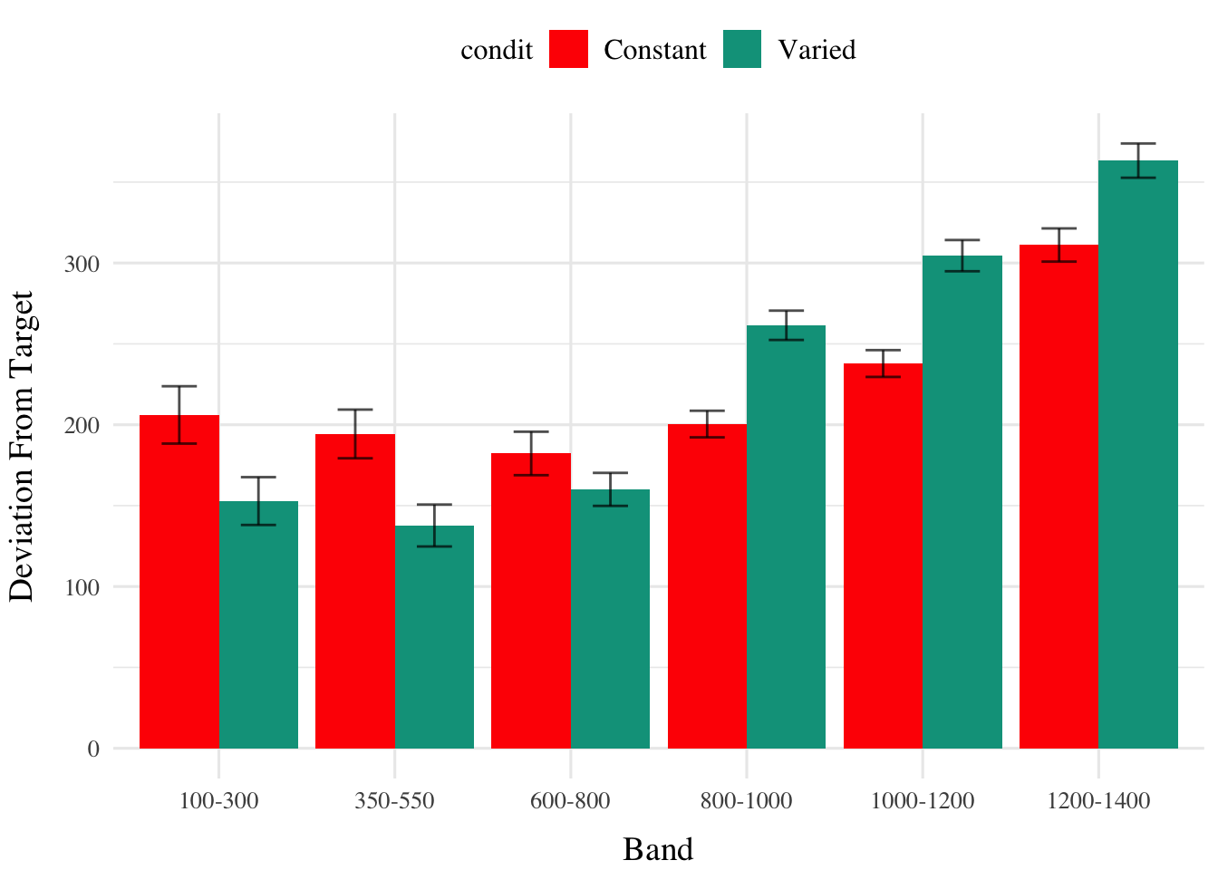
Deviation From Target Band
Descriptive summaries testing deviation data are provided in Table 1 and Figure 2. To model differences in accuracy between groups, we used Bayesian mixed effects regression models to the trial level data from the testing phase. The primary model predicted the absolute deviation from the target velocity band (dist) as a function of training condition (condit), target velocity band (band), and their interaction, with random intercepts and slopes for each participant (id).
Table 2: Experiment 2. Bayesian Mixed Model predicting absolute deviation as a function of condition (Constant vs. Varied) and Velocity Band
Term
Estimate
95% CrI Lower
95% CrI Upper
pd
Intercept
151.71
90.51
215.86
1.00
conditVaried
-70.33
-156.87
16.66
0.94
Band
0.10
0.02
0.18
1.00
condit*Band
0.12
0.02
0.23
0.99
Contrasts
contrast
Band
value
lower
upper
pd
Constant - Varied
100
57.57
-20.48
135.32
0.93
Constant - Varied
350
26.60
-30.93
83.84
0.83
Constant - Varied
600
-4.30
-46.73
38.52
0.58
Constant - Varied
800
-29.30
-69.38
11.29
0.92
Constant - Varied
1000
-54.62
-101.06
-5.32
0.98
Constant - Varied
1200
-79.63
-139.47
-15.45
0.99
The model predicting absolute deviation showed a modest tendency for the varied training group to have lower deviation compared to the constant training group (β = -70.33, 95% CI [-156.87, 16.66]),with 94% of the posterior distribution being less than 0. This suggests a potential benefit of training with variation, though the evidence is not definitive.
(SHOULD PROBABLY DO ALTERNATE ANALYSIS THAT ONLY CONSIDERS THE NOVEL EXTRAPOLATION BANDS)
Code
condEffects<-function(m){m|>ggplot(aes(x =bandInt, y =.value, color =condit, fill =condit))+stat_dist_pointinterval()+stat_halfeye(alpha=.2)+stat_lineribbon(alpha =.25, size =1, .width =c(.95))+theme(axis.text.x =element_text(angle =45, hjust =0.5, vjust =0.5))+ylab("Predicted X Velocity")+xlab("Band")}e2_distBMM|>emmeans(~condit+bandInt, at =list(bandInt =c(100, 350, 600, 800, 1000, 1200)))|>gather_emmeans_draws()|>condEffects()+scale_x_continuous(breaks =c(100, 350, 600, 800, 1000, 1200), labels =levels(testE2$vb), limits =c(0, 1400))
Figure 4: E2. Conditioinal Effect of Training Condition and Band. Ribbon indicated 95% Credible Intervals.
Discrimination between Velocity Bands
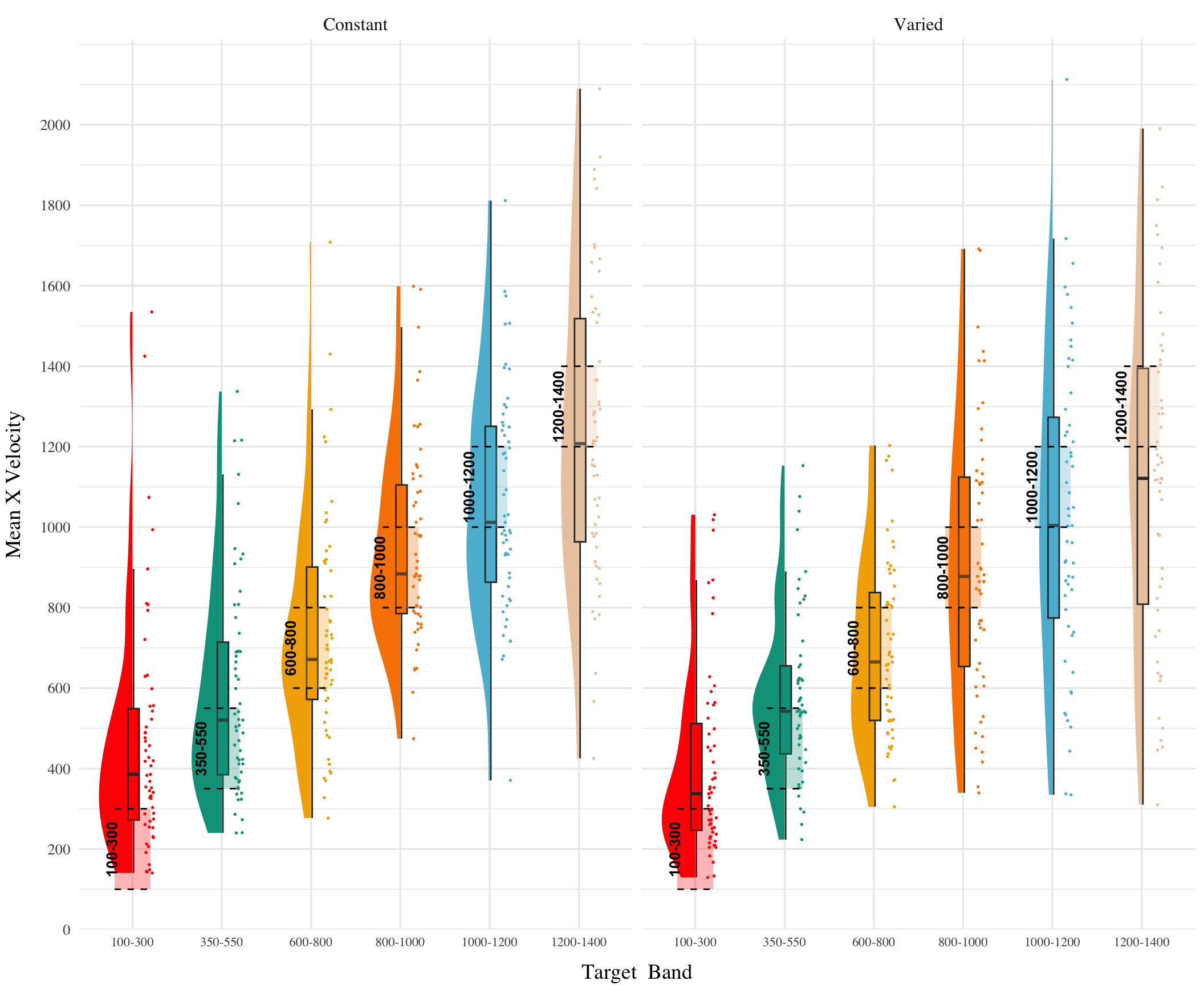
In addition to accuracy/deviation. We also assessed the ability of participants to reliably discriminate between the velocity bands (i.e. responding differently when prompted for band 600-800 than when prompted for band 150-350). Table 3 shows descriptive statistics of this measure, and Figure 1 visualizes the full distributions of throws for each combination of condition and velocity band. To quantify discrimination, we again fit Bayesian Mixed Models as above, but this time the dependent variable was the raw x velocity generated by participants.
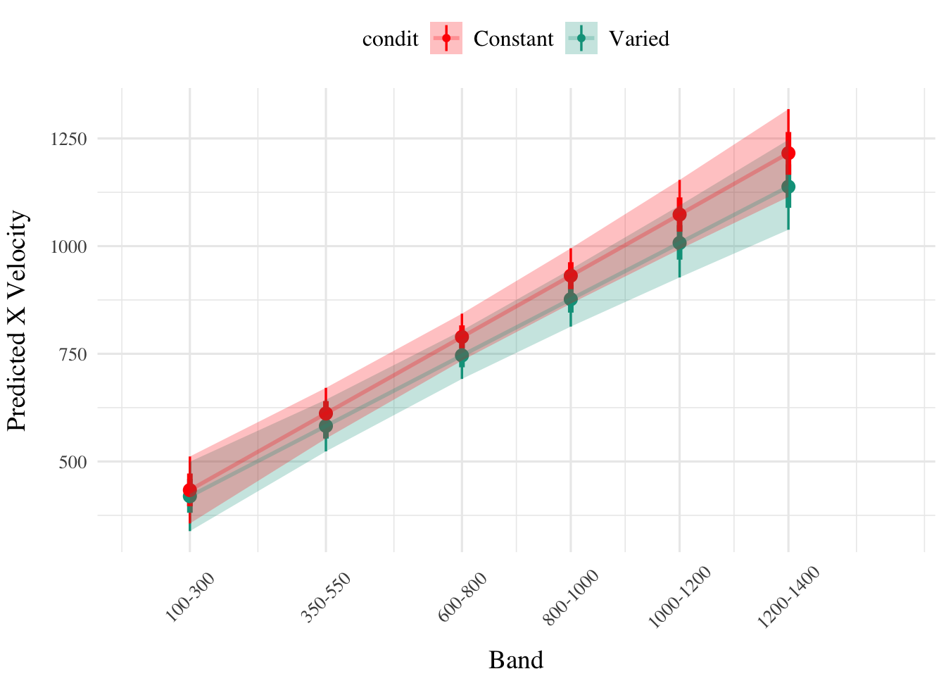
When examining discrimination ability using the model predicting raw x-velocity, the results were less clear than those of the absolute deviation analysis. The slope on Velocity Band (β = 0.71, 95% CrI [0.58, 0.84]) indicates that participants showed good discrimination between bands overall. However, the interaction term suggested this effect was not modulated by training condition (β = -0.06, 95% CrI [-0.24, 0.13]) Thus, while varied training may provide some advantage for accuracy, both training conditions seem to have similar abilities to discriminate between velocity bands.
Code
e2_vxBMM|>emmeans(~condit+bandInt, at =list(bandInt =c(100, 350, 600, 800, 1000, 1200)))|>gather_emmeans_draws()|>ggplot(aes(x =bandInt, y =.value, color =condit, fill =condit))+stat_dist_pointinterval()+stat_lineribbon(alpha =.25, size =1, .width =c(.95))+ylab("Predicted X Velocity")+xlab("Band")+scale_x_continuous(breaks =c(100, 350, 600, 800, 1000, 1200), labels =levels(testE2$vb), limits =c(0, 1400))+theme(axis.text.x =element_text(angle =45, hjust =0.5, vjust =0.5))
Figure 6: Conditional effect of training condition and Band. Ribbons indicate 95% HDI.
indvDraws<-left_join(random_effects, fixed_effects, by =join_by(".chain", ".iteration", ".draw"))|>rename(bandInt_RF =bandInt,RF_Intercept=Intercept)|>right_join(new_data_grid, by =join_by("id"))|>mutate( Slope =bandInt_RF+b_bandInt, Intercept=RF_Intercept+b_Intercept, estimate =(b_Intercept+RF_Intercept)+(bandInt*(b_bandInt+bandInt_RF))+(bandInt*condit_dummy)*`b_conditVaried:bandInt`, SlopeInt =Slope+(`b_conditVaried:bandInt`*condit_dummy))
Warning in right_join(rename(left_join(random_effects, fixed_effects, by = join_by(".chain", : Detected an unexpected many-to-many relationship between `x` and `y`.
ℹ Row 1 of `x` matches multiple rows in `y`.
ℹ Row 1 of `y` matches multiple rows in `x`.
ℹ If a many-to-many relationship is expected, set `relationship =
  "many-to-many"` to silence this warning.
Table 5: Slope coefficients by quartile, per condition
Condition
Q_0%_mean
Q_25%_mean
Q_50%_mean
Q_75%_mean
Q_100%_mean
Constant
-0.2788310
0.3898592
0.697289
1.0778097
1.616840
Varied
-0.2454246
0.3040574
0.679329
0.9470274
1.810293
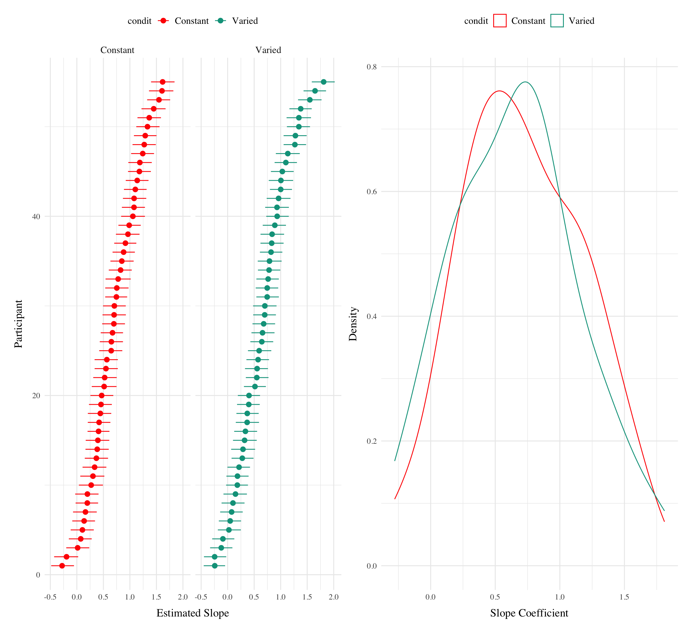
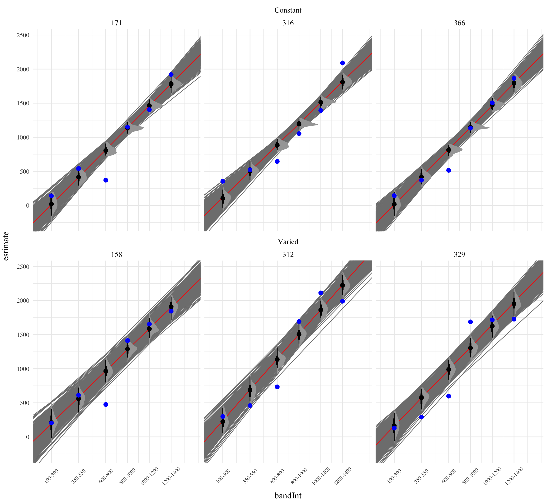
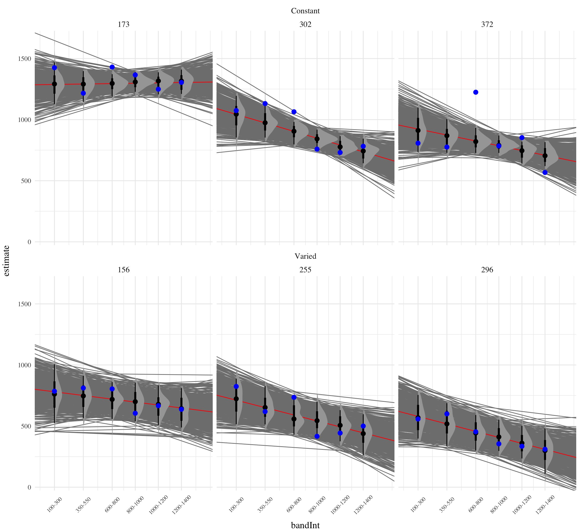
Figure 7 visually represents the distributions of estimated slopes relating velocity band to x velocity for each participant, ordered from lowest to highest within condition. Slope values are lower overall for varied training compared to constant training. Figure Xb plots the density of these slopes for each condition. The distribution for varied training has more mass at lower values than the constant training distribution. Both figures illustrate the model’s estimate that varied training resulted in less discrimination between velocity bands, evidenced by lower slopes on average.
Figure 8: Subset of Varied and Constant Participants with the smallest and largest estimated slope values. Red lines represent the best fitting line for each participant, gray lines are 200 random samples from the posterior distribution. Colored points and intervals at each band represent the empirical median and 95% HDI.
testE2|>ggplot(aes(x=train_end,y=dist,fill=condit))+stat_summary(geom ="line", position=position_dodge(), fun =mean)+stat_summary(geom ="errorbar", position=position_dodge(.9), fun.data =mean_se, width =.4, alpha =.7)+facet_wrap(~vb)+labs(x="Band", y="Deviation From Target")
Warning: Width not defined
ℹ Set with `position_dodge(width = ...)`
Warning: `position_dodge()` requires non-overlapping x intervals.
`position_dodge()` requires non-overlapping x intervals.
`position_dodge()` requires non-overlapping x intervals.
`position_dodge()` requires non-overlapping x intervals.
`position_dodge()` requires non-overlapping x intervals.
`position_dodge()` requires non-overlapping x intervals.
Code
testE2|>ggplot(aes(x=train_end,y=dist,fill=condit,col=condit))+#geom_point() +geom_smooth(method="loess")+facet_wrap(~vb)+labs(x="Band", y="Deviation From Target")
`geom_smooth()` using formula = 'y ~ x'
Code
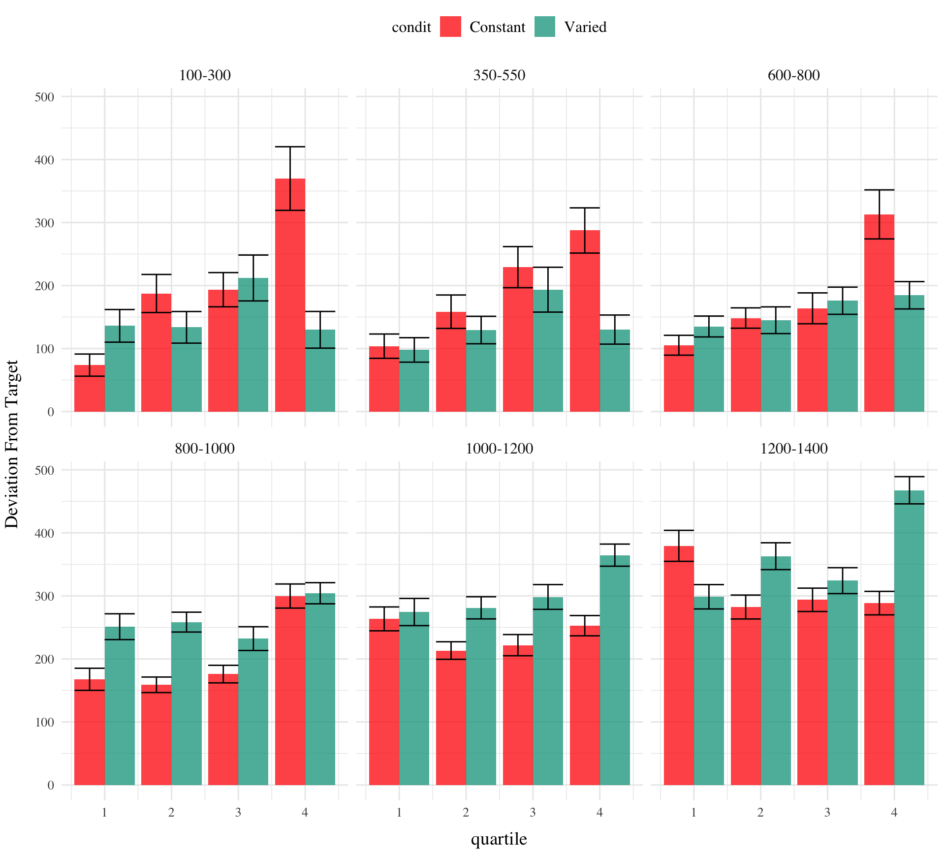
# create quartiles for train_endtestE2|>group_by(condit,vb)|>mutate(train_end_q =ntile(train_end,4))|>ggplot(aes(x=train_end_q,y=dist,fill=condit))+stat_bar+facet_wrap(~vb)+labs(x="quartile", y="Deviation From Target")
Code
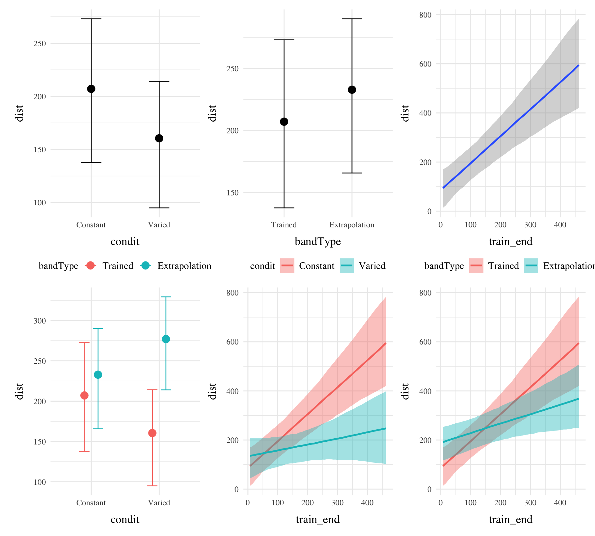
bmtd3<-brm(dist~condit*bandType*train_end+(1|bandInt)+(1|id), data=testE2, file=paste0(here::here("data/model_cache","e2_trainEnd_BT_RF2")), iter=1000,chains=2, control =list(adapt_delta =.92, max_treedepth =11))summary(bmtd3)
 Family: gaussian
  Links: mu = identity; sigma = identity
Formula: dist ~ condit * bandType * train_end + (1 | bandInt) + (1 | id)
   Data: testE2 (Number of observations: 6709)
  Draws: 2 chains, each with iter = 1000; warmup = 500; thin = 1;
         total post-warmup draws = 1000

Group-Level Effects:
~bandInt (Number of levels: 6)
              Estimate Est.Error l-95% CI u-95% CI Rhat Bulk_ESS Tail_ESS
sd(Intercept)    56.29     23.16    27.44   117.13 1.01      368      453

~id (Number of levels: 110)
              Estimate Est.Error l-95% CI u-95% CI Rhat Bulk_ESS Tail_ESS
sd(Intercept)    96.88      7.59    83.12   112.62 1.00      238      391

Population-Level Effects:
                                             Estimate Est.Error l-95% CI
Intercept                                       85.19     40.60     2.29
conditVaried                                    46.19     40.72   -31.33
bandTypeExtrapolation                          101.67     27.77    49.32
train_end                                        1.10      0.23     0.67
conditVaried:bandTypeExtrapolation             -11.41     31.46   -74.92
conditVaried:train_end                          -0.85      0.32    -1.51
bandTypeExtrapolation:train_end                 -0.69      0.19    -1.06
conditVaried:bandTypeExtrapolation:train_end     0.93      0.23     0.46
                                             u-95% CI Rhat Bulk_ESS Tail_ESS
Intercept                                      163.45 1.01      222      298
conditVaried                                   127.49 1.01      237      363
bandTypeExtrapolation                          159.00 1.00      490      727
train_end                                        1.59 1.00      289      372
conditVaried:bandTypeExtrapolation              48.65 1.00      485      722
conditVaried:train_end                          -0.23 1.01      242      417
bandTypeExtrapolation:train_end                 -0.34 1.00      402      646
conditVaried:bandTypeExtrapolation:train_end     1.35 1.00      385      602

Family Specific Parameters:
      Estimate Est.Error l-95% CI u-95% CI Rhat Bulk_ESS Tail_ESS
sigma   241.83      2.08   237.75   245.98 1.00     1779      602

Draws were sampled using sample(hmc). For each parameter, Bulk_ESS
and Tail_ESS are effective sample size measures, and Rhat is the potential
scale reduction factor on split chains (at convergence, Rhat = 1).
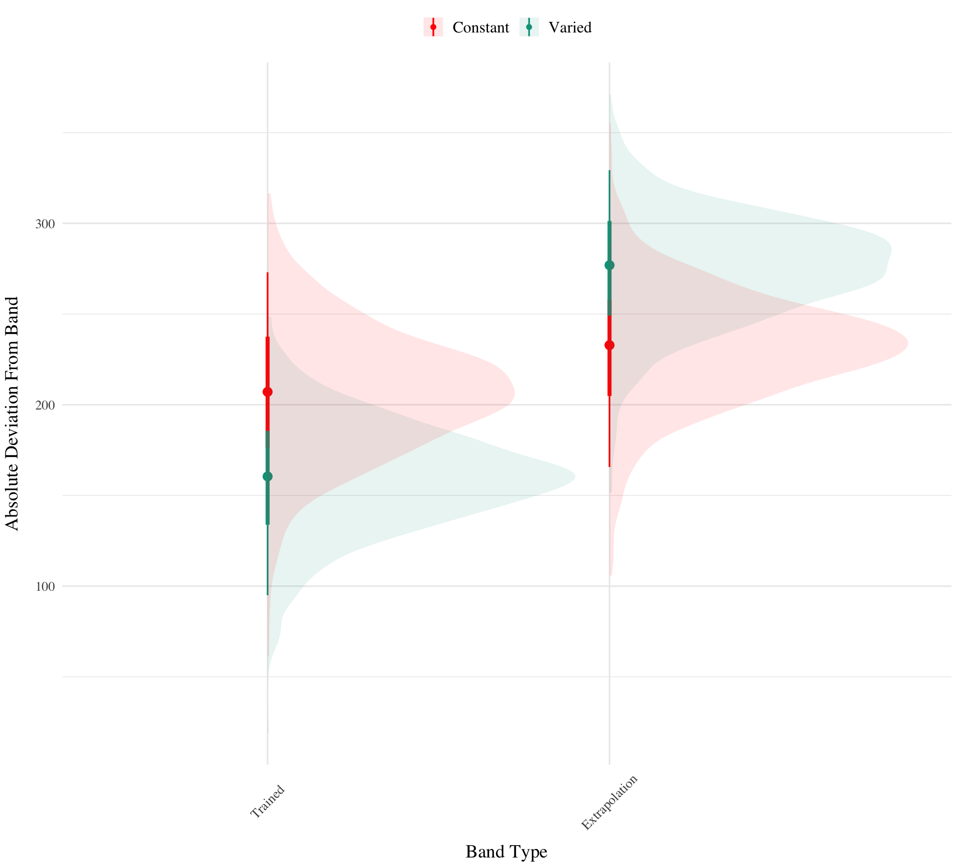
condEffects<-function(m,xvar){m|>ggplot(aes(x ={{xvar}}, y =.value, color =condit, fill =condit))+stat_dist_pointinterval()+stat_halfeye(alpha=.1, height=.5)+theme(legend.title=element_blank(),axis.text.x =element_text(angle =45, hjust =0.5, vjust =0.5))}bmtd3|>emmeans(~condit*bandType*train_end)|>gather_emmeans_draws()|>condEffects(bandType)+labs(y="Absolute Deviation From Band", x="Band Type")
---title: "HTW E2 Testing"categories: [Analyses, R, Bayesian]lightbox: truepage-layout: fulltoc: falsecode-fold: truecode-tools: true---```{r setup2b, include=FALSE}source(here::here("Functions", "packages.R"))options(brms.backend="cmdstanr",mc.cores=4)e2 <- readRDS(here("data/e2_08-04-23.rds")) testE2 <- e2 |> filter(expMode2=="Test")e2Sbjs <- testE2 |> group_by(id,condit) |> summarise(n=n())testE2Avg <- testE2 %>% group_by(id, condit, vb, bandInt,bandType,tOrder) %>% summarise(nHits=sum(dist==0),vx=mean(vx),dist=mean(dist),sdist=mean(sdist),n=n(),Percent_Hit=nHits/n)nbins=5trainE2 <- e2 |> filter(expMode2=="Train") |> group_by(id,condit, vb) |> mutate(Trial_Bin = cut( gt.train, breaks = seq(1, max(gt.train),length.out=nbins+1),include.lowest = TRUE, labels=FALSE)) trainE2_max <- trainE2 |> filter(Trial_Bin == nbins, bandInt==600)trainE2_avg <- trainE2_max |> group_by(id,condit) |> summarise(avg = mean(dist))nbins=5trainE2 <- e2 |> filter(expMode2=="Train") |> group_by(id,condit, vb) |> mutate(Trial_Bin = cut( gt.bandStage, breaks = seq(1, max(gt.bandStage),length.out=nbins+1),include.lowest = TRUE, labels=FALSE)) trainE2_max <- trainE2 |> filter(Trial_Bin == nbins, bandInt==600)trainE2_avg <- trainE2_max |> group_by(id,condit) |> summarise(train_end = mean(dist))trainE2 |> select(id,condit,Trial_Bin,trial,vb,bandInt,dist,vx,gt.bandStage) |> group_by(id,condit,vb,Trial_Bin) |> summarise(mean_dist=mean(dist),mean_vx=mean(vx),n=n()) testE2 <- testE2 |> left_join(trainE2_avg, by=c("id","condit")) ```@fig-design-e2 illustrates the design of Experiment 2. The stages of the experiment (i.e. training, testing no-feedback, test with feedback), are identical to that of Experiment 1. The only change is that Experiment 2 participants train, and then test, on bands in the reverse order of Experiment 1 (i.e. training on the softer bands; and testing on the harder bands). ```{dot}//| label: fig-design-e2//| fig-cap: "Experiment 2 Design. Constant and Varied participants complete different training conditions. The training and testing bands are the reverse of Experiment 1. "//| fig-width: 8.0//| fig-height: 2.5//| fig-responsive: false//| column: screen-inset-rightdigraph { graph [layout = dot, rankdir = LR] node [shape = rectangle, style = filled] data1 [label = " Varied Training \n100-300\n350-550\n600-800", fillcolor = "#FF0000"] data2 [label = " Constant Training \n600-800", fillcolor = "#00A08A"] Test3 [label = " Final Test \n Novel With Feedback \n800-1000\n1000-1200\n1200-1400", fillcolor = "#ECCBAE"] data1 -> Test1 data2 -> Test1 subgraph cluster { label = "Test Phase \n(Counterbalanced Order)" Test1 [label = "Test \nNovel Bands \n800-1000\n1000-1200\n1200-1400", fillcolor = "#ECCBAE"] Test2 [label = " Test \n Varied Training Bands \n100-300\n350-550\n600-800", fillcolor = "#ECCBAE"] Test1 -> Test2 } Test2 -> Test3}```### Results#### Testing Phase - No feedback. In the first part of the testing phase, participants are tested from each of the velocity bands, and receive no feedback after each throw. ##### Deviation From Target BandDescriptive summaries testing deviation data are provided in @tbl-e2-test-nf-deviation and @fig-e2-test-dev. To model differences in accuracy between groups, we used Bayesian mixed effects regression models to the trial level data from the testing phase. The primary model predicted the absolute deviation from the target velocity band (dist) as a function of training condition (condit), target velocity band (band), and their interaction, with random intercepts and slopes for each participant (id). \begin{equation}dist_{ij} = \beta_0 + \beta_1 \cdot condit_{ij} + \beta_2 \cdot band_{ij} + \beta_3 \cdot condit_{ij} \cdot band_{ij} + b_{0i} + b_{1i} \cdot band_{ij} + \epsilon_{ij}\end{equation}```{r}#| label: tbl-e2-test-nf-deviation#| tbl-cap: "Testing Deviation - Empirical Summary"#| tbl-subcap: ["Constant Testing - Deviation", "Varied Testing - Deviation"]result <-test_summary_table(testE2, "dist","Deviation", mfun =list(mean = mean, median = median, sd = sd))result$constant |>kable()result$varied |>kable()# make kable table with smaller font size# result$constant |> kbl(caption="Constant Testing - Deviation",booktabs=T,escape=F) |> kable_styling(font_size = 7)``````{r}#| label: fig-e2-test-dev#| fig-cap: E2. Deviations from target band during testing without feedback stage. testE2 |>ggplot(aes(x = vb, y = dist,fill=condit)) +stat_summary(geom ="bar", position=position_dodge(), fun = mean) +stat_summary(geom ="errorbar", position=position_dodge(.9), fun.data = mean_se, width = .4, alpha = .7) +labs(x="Band", y="Deviation From Target")``````{r}#options(brms.backend="cmdstanr",mc.cores=4)modelFile <-paste0(here::here("data/model_cache/"), "e2_dist_Cond_Type_RF_2")bmtd2 <-brm(dist ~ condit * bandType + (1|bandInt) + (1|id), data=testE2, file=modelFile,iter=5000,chains=4, control =list(adapt_delta = .94, max_treedepth =13))#bayestestR::describe_posterior(bmtd)mted2 <-as.data.frame(describe_posterior(bmtd2, centrality ="Mean"))[, c(1,2,4,5,6)]colnames(mted2) <-c("Term", "Estimate","95% CrI Lower", "95% CrI Upper", "pd")mted2 |>mutate(across(where(is.numeric), \(x) round(x, 2))) |> tibble::remove_rownames() |>mutate(Term = stringr::str_remove(Term, "b_")) |>kable(booktabs=TRUE) ``````{r}#| label: fig-e2-test-dev2#| fig-cap: E2. Deviations from target band during testing without feedback stage. pe1td <- testE2 |>ggplot(aes(x = vb, y = dist,fill=condit)) +stat_summary(geom ="bar", position=position_dodge(), fun = mean) +stat_summary(geom ="errorbar", position=position_dodge(.9), fun.data = mean_se, width = .4, alpha = .7) +theme(legend.title=element_blank(),axis.text.x =element_text(angle =45, hjust =0.5, vjust =0.5)) +labs(x="Band", y="Deviation From Target")condEffects <-function(m,xvar){ m |>ggplot(aes(x = {{xvar}}, y = .value, color = condit, fill = condit)) +stat_dist_pointinterval() +stat_halfeye(alpha=.1, height=.5) +theme(legend.title=element_blank(),axis.text.x =element_text(angle =45, hjust =0.5, vjust =0.5)) }pe1ce <- bmtd2 |>emmeans( ~condit + bandType) |>gather_emmeans_draws() |>condEffects(bandType) +labs(y="Absolute Deviation From Band", x="Band Type")(pe1td + pe1ce) +plot_annotation(tag_levels='A')``````{r}#| label: tbl-e2-bmm-dist#| tbl-cap: "Experiment 2. Bayesian Mixed Model predicting absolute deviation as a function of condition (Constant vs. Varied) and Velocity Band"#contrasts(test$condit) # contrasts(testE2$vb)modelName <-"e2_testDistBand_RF_5K"e2_distBMM <-brm(dist ~ condit * bandInt + (1+ bandInt|id),data=testE2,file=paste0(here::here("data/model_cache",modelName)),iter=5000,chains=4)mp2 <-GetModelStats(e2_distBMM) |>kable(escape=F,booktabs=T)mp2e2_distBMM |>emmeans("condit",by="bandInt",at=list(bandInt=c(100,350,600,800,1000,1200)),epred =TRUE, re_formula =NA) |>pairs() |>gather_emmeans_draws() |>summarize(median_qi(.value),pd=sum(.value>0)/n()) |>select(contrast,Band=bandInt,value=y,lower=ymin,upper=ymax,pd) |>mutate(across(where(is.numeric), \(x) round(x, 2)),pd=ifelse(value<0,1-pd,pd)) |>kable(caption="Contrasts")coef_details <-get_coef_details(e2_distBMM, "conditVaried")```The model predicting absolute deviation showed a modest tendency for the varied training group to have lower deviation compared to the constant training group (β = `r coef_details$estimate`, 95% CI \[`r coef_details$conf.low`, `r coef_details$conf.high`\]),with 94% of the posterior distribution being less than 0. This suggests a potential benefit of training with variation, though the evidence is not definitive.(SHOULD PROBABLY DO ALTERNATE ANALYSIS THAT ONLY CONSIDERS THE NOVEL EXTRAPOLATION BANDS)```{r}#| label: fig-e2-bmm-dist#| fig-cap: E2. Conditioinal Effect of Training Condition and Band. Ribbon indicated 95% Credible Intervals. condEffects <-function(m){ m |>ggplot(aes(x = bandInt, y = .value, color = condit, fill = condit)) +stat_dist_pointinterval() +stat_halfeye(alpha=.2) +stat_lineribbon(alpha = .25, size =1, .width =c(.95)) +theme(axis.text.x =element_text(angle =45, hjust =0.5, vjust =0.5)) +ylab("Predicted X Velocity") +xlab("Band")}e2_distBMM |>emmeans( ~condit + bandInt, at =list(bandInt =c(100, 350, 600, 800, 1000, 1200))) |>gather_emmeans_draws() |>condEffects()+scale_x_continuous(breaks =c(100, 350, 600, 800, 1000, 1200), labels =levels(testE2$vb), limits =c(0, 1400)) ```##### Discrimination between Velocity BandsIn addition to accuracy/deviation. We also assessed the ability of participants to reliably discriminate between the velocity bands (i.e. responding differently when prompted for band 600-800 than when prompted for band 150-350). @tbl-e2-test-nf-vx shows descriptive statistics of this measure, and Figure 1 visualizes the full distributions of throws for each combination of condition and velocity band. To quantify discrimination, we again fit Bayesian Mixed Models as above, but this time the dependent variable was the raw x velocity generated by participants. \begin{equation}vx_{ij} = \beta_0 + \beta_1 \cdot condit_{ij} + \beta_2 \cdot bandInt_{ij} + \beta_3 \cdot condit_{ij} \cdot bandInt_{ij} + b_{0i} + b_{1i} \cdot bandInt_{ij} + \epsilon_{ij}\end{equation}```{r}#| label: fig-e2-test-vx#| fig-cap: E2 testing x velocities. Translucent bands with dash lines indicate the correct range for each velocity band. #| fig-width: 11#| fig-height: 9testE2 %>%group_by(id,vb,condit) |>plot_distByCondit()``````{r}#| label: tbl-e2-test-nf-vx#| tbl-cap: "Testing vx - Empirical Summary"#| tbl-subcap: ["Constant Testing - vx", "Varied Testing - vx"]#| layout-ncol: 1result <-test_summary_table(testE2, "vx","X Velocity" ,mfun =list(mean = mean, median = median, sd = sd))result$constant |>kable()result$varied |>kable()``````{r}#| label: tbl-e2-bmm-vx#| tbl-cap: "Experiment 2. Bayesian Mixed Model Predicting Vx as a function of condition (Constant vs. Varied) and Velocity Band"e2_vxBMM <-brm(vx ~ condit * bandInt + (1+ bandInt|id),data=testE2,file=paste0(here::here("data/model_cache", "e2_testVxBand_RF_5k")),iter=5000,chains=4,silent=0,control=list(adapt_delta=0.94, max_treedepth=13))mt3 <-GetModelStats(e2_vxBMM ) |>kable(escape=F,booktabs=T)mt3cd1 <-get_coef_details(e2_vxBMM, "conditVaried")sc1 <-get_coef_details(e2_vxBMM, "bandInt")intCoef1 <-get_coef_details(e2_vxBMM, "conditVaried:bandInt")```See @tbl-e2-bmm-vx for the full model results. When examining discrimination ability using the model predicting raw x-velocity, the results were less clear than those of the absolute deviation analysis. The slope on Velocity Band (β = `r sc1$estimate`, 95% CrI \[`r sc1$conf.low`, `r sc1$conf.high`\]) indicates that participants showed good discrimination between bands overall. However, the interaction term suggested this effect was not modulated by training condition (β = `r intCoef1$estimate`, 95% CrI \[`r intCoef1$conf.low`, `r intCoef1$conf.high`\]) Thus, while varied training may provide some advantage for accuracy, both training conditions seem to have similar abilities to discriminate between velocity bands.```{r}#| label: fig-e2-bmm-vx#| fig-cap: Conditional effect of training condition and Band. Ribbons indicate 95% HDI. e2_vxBMM |>emmeans( ~condit + bandInt, at =list(bandInt =c(100, 350, 600, 800, 1000, 1200))) |>gather_emmeans_draws() |>ggplot(aes(x = bandInt, y = .value, color = condit, fill = condit)) +stat_dist_pointinterval() +stat_lineribbon(alpha = .25, size =1, .width =c(.95)) +ylab("Predicted X Velocity") +xlab("Band")+scale_x_continuous(breaks =c(100, 350, 600, 800, 1000, 1200), labels =levels(testE2$vb), limits =c(0, 1400)) +theme(axis.text.x =element_text(angle =45, hjust =0.5, vjust =0.5)) ``````{r}#| label: fig-e2-slope-dist#| fig-cap: Subset of Varied and Constant Participants with the largest estimated slope values. Red lines represent the best fitting line for each participant, gray lines are 100 random samples from the posterior distribution. Colored points and intervals at each band represent the empirical median and 95% HDI. #| fig-height: 9#| fig-width: 10#| eval: falsenew_data_grid=map_dfr(1, ~data.frame(unique(testE2[,c("id","condit","bandInt")]))) |> dplyr::arrange(id,bandInt) |>mutate(condit_dummy =ifelse(condit =="Varied", 1, 0)) indv_coefs <-coef(e2_vxBMM)$id |>as_tibble(rownames="id") |>select(id, starts_with("Est")) |>left_join(e2Sbjs, by=join_by(id) ) |>group_by(condit) |>mutate(rank =rank(desc(Estimate.bandInt)),intErrorRank=rank((Est.Error.Intercept)),bandErrorRank=rank((Est.Error.bandInt)),nCond =n()) |>arrange(intErrorRank)fixed_effects <- e2_vxBMM |>spread_draws(`^b_.*`,regex=TRUE) |>arrange(.chain,.draw,.iteration)random_effects <- e2_vxBMM |>gather_draws(`^r_id.*$`, regex =TRUE, ndraws =2000) |>separate(.variable, into =c("effect", "id", "term"), sep ="\\[|,|\\]") |>mutate(id =factor(id,levels=levels(testE2$id))) |>pivot_wider(names_from = term, values_from = .value) |>arrange(id,.chain,.draw,.iteration)cd <-left_join(random_effects, fixed_effects, by =join_by(".chain", ".iteration", ".draw")) |>rename(bandInt_RF = bandInt) |>mutate(Slope=bandInt_RF+b_bandInt) |>group_by(id) cdMed <- cd |>group_by(id) |>median_qi(Slope) |>left_join(e2Sbjs, by=join_by(id)) |>group_by(condit) |>mutate(rankSlope=rank(Slope)) |>arrange(rankSlope)cdMed %>%ggplot(aes(y=rankSlope, x=Slope,fill=condit,color=condit)) +geom_pointrange(aes(xmin=.lower , xmax=.upper)) +labs(x="Estimated Slope", y="Participant") +facet_wrap(~condit) # cdMed |> ggplot(aes(x = condit, y = Slope,fill=condit)) +# stat_summary(geom = "bar", position=position_dodge(), fun = mean) +# stat_summary(geom = "errorbar", position=position_dodge(.9), fun.data = mean_se, width = .4, alpha = .7) + # geom_jitter()# labs(x="Band", y="Deviation From Target")``````{r}#| label: tbl-e2-slope-quartile#| tbl-cap: "Slope coefficients by quartile, per condition"new_data_grid=map_dfr(1, ~data.frame(unique(testE2[,c("id","condit","bandInt")]))) |> dplyr::arrange(id,bandInt) |>mutate(condit_dummy =ifelse(condit =="Varied", 1, 0)) indv_coefs <-as_tibble(coef(e2_vxBMM)$id, rownames="id")|>select(id, starts_with("Est")) |>left_join(e2Sbjs, by=join_by(id) ) fixed_effects <- e2_vxBMM |>spread_draws(`^b_.*`,regex=TRUE) |>arrange(.chain,.draw,.iteration)random_effects <- e2_vxBMM |>gather_draws(`^r_id.*$`, regex =TRUE, ndraws =1500) |>separate(.variable, into =c("effect", "id", "term"), sep ="\\[|,|\\]") |>mutate(id =factor(id,levels=levels(testE2$id))) |>pivot_wider(names_from = term, values_from = .value) |>arrange(id,.chain,.draw,.iteration) indvDraws <-left_join(random_effects, fixed_effects, by =join_by(".chain", ".iteration", ".draw")) |>rename(bandInt_RF = bandInt,RF_Intercept=Intercept) |>right_join(new_data_grid, by =join_by("id")) |>mutate(Slope = bandInt_RF+b_bandInt,Intercept= RF_Intercept + b_Intercept,estimate = (b_Intercept + RF_Intercept) + (bandInt*(b_bandInt+bandInt_RF)) + (bandInt * condit_dummy) *`b_conditVaried:bandInt`,SlopeInt = Slope + (`b_conditVaried:bandInt`*condit_dummy) ) indvSlopes <- indvDraws |>group_by(id) |>median_qi(Slope,SlopeInt, Intercept,b_Intercept,b_bandInt) |>left_join(e2Sbjs, by=join_by(id)) |>group_by(condit) |>select(id,condit,Intercept,b_Intercept,starts_with("Slope"),b_bandInt, n) |>mutate(rankSlope=rank(Slope)) |>arrange(rankSlope) |>ungroup() indvSlopes |>mutate(Condition=condit) |>group_by(Condition) |>reframe(enframe(quantile(SlopeInt, c(0.0,0.25, 0.5, 0.75,1)), "quantile", "SlopeInt")) |>pivot_wider(names_from=quantile,values_from=SlopeInt,names_prefix="Q_") |>group_by(Condition) |>summarise(across(starts_with("Q"), list(mean = mean))) |>kable()```@fig-e2-bmm-bx2 visually represents the distributions of estimated slopes relating velocity band to x velocity for each participant, ordered from lowest to highest within condition. Slope values are lower overall for varied training compared to constant training. Figure Xb plots the density of these slopes for each condition. The distribution for varied training has more mass at lower values than the constant training distribution. Both figures illustrate the model's estimate that varied training resulted in less discrimination between velocity bands, evidenced by lower slopes on average.```{r}#| label: fig-e2-bmm-bx2#| fig-cap: Slope distributions between condition#| fig-subcap: ["Slope estimates by participant - ordered from lowest to highest within each condition. ", "Destiny of slope coefficients by training group"]#| fig-height: 11#| fig-width: 12 indvSlopes |>ggplot(aes(y=rankSlope, x=SlopeInt,fill=condit,color=condit)) +geom_pointrange(aes(xmin=SlopeInt.lower , xmax=SlopeInt.upper)) +labs(x="Estimated Slope", y="Participant") +facet_wrap(~condit) +ggplot(indvSlopes, aes(x = SlopeInt, color = condit)) +geom_density() +labs(x="Slope Coefficient",y="Density")``````{r}#| label: fig-e2-indv-slopes#| fig-cap: Subset of Varied and Constant Participants with the smallest and largest estimated slope values. Red lines represent the best fitting line for each participant, gray lines are 200 random samples from the posterior distribution. Colored points and intervals at each band represent the empirical median and 95% HDI. #| fig-subcap: ["subset with largest slopes", "subset with smallest slopes"]#| fig-height: 11#| fig-width: 12nSbj <-3indvDraws |>indv_model_plot(indvSlopes, testE2Avg, SlopeInt,rank_variable=Slope,n_sbj=nSbj,"max")indvDraws |>indv_model_plot(indvSlopes, testE2Avg,SlopeInt, rank_variable=Slope,n_sbj=nSbj,"min")```### control for training end performance```{r}#| fig-height: 9#| fig-width: 10testE2 |>group_by(id,condit) |>pivot_longer(c("dist","train_end"),names_to="var",values_to="value") |>ggplot(aes(x=var,y=value, fill=condit)) + stat_bar +facet_wrap(~var)testE2 |>ggplot(aes(x=train_end,y=dist,fill=condit)) +stat_summary(geom ="line", position=position_dodge(), fun = mean) +stat_summary(geom ="errorbar", position=position_dodge(.9), fun.data = mean_se, width = .4, alpha = .7) +facet_wrap(~vb) +labs(x="Band", y="Deviation From Target")testE2 |>ggplot(aes(x=train_end,y=dist,fill=condit,col=condit)) +#geom_point() +geom_smooth(method="loess") +facet_wrap(~vb) +labs(x="Band", y="Deviation From Target")# create quartiles for train_endtestE2 |>group_by(condit,vb) |>mutate(train_end_q =ntile(train_end,4)) |>ggplot(aes(x=train_end_q,y=dist,fill=condit)) + stat_bar +facet_wrap(~vb) +labs(x="quartile", y="Deviation From Target")``````{r}#| fig-height: 9#| fig-width: 10#| bmtd3 <-brm(dist ~ condit * bandType * train_end + (1|bandInt) + (1|id), data=testE2, file=paste0(here::here("data/model_cache","e2_trainEnd_BT_RF2")),iter=1000,chains=2, control =list(adapt_delta = .92, max_treedepth =11))summary(bmtd3)bayestestR::describe_posterior(bmtd3)condEffects <-function(m,xvar){ m |>ggplot(aes(x = {{xvar}}, y = .value, color = condit, fill = condit)) +stat_dist_pointinterval() +stat_halfeye(alpha=.1, height=.5) +theme(legend.title=element_blank(),axis.text.x =element_text(angle =45, hjust =0.5, vjust =0.5)) } bmtd3 |>emmeans( ~condit * bandType * train_end) |>gather_emmeans_draws() |>condEffects(bandType) +labs(y="Absolute Deviation From Band", x="Band Type")ce_bmtd3 <-plot(conditional_effects(bmtd3),points=FALSE,plot=FALSE)wrap_plots(ce_bmtd3)```