HTW E1 Testing

Analyses Strategy

All data processing and statistical analyses were performed in R version 4.31 Team (2020). To assess differences between groups, we used Bayesian Mixed Effects Regression. Model fitting was performed with the brms package in R Bürkner (2017), and descriptive stats and tables were extracted with the BayestestR package Makowski et al. (2019). Mixed effects regression enables us to take advantage of partial pooling, simultaneously estimating parameters at the individual and group level. Our use of Bayesian, rather than frequentist methods allows us to directly quantify the uncertainty in our parameter estimates, as well as circumventing convergence issues common to the frequentist analogues of our mixed models. For each model, we report the median values of the posterior distribution, and 95% credible intervals.

Each model was set to run with 4 chains, 5000 iterations per chain, with the first 2500 of which were discarded as warmup chains. Rhat values were generally within an acceptable range, with values <=1.02 (see appendix for diagnostic plots). We used uninformative priors for the fixed effects of the model (condition and velocity band), and weakly informative Student T distributions for for the random effects.

We compared varied and constant performance across two measures, deviation and discrimination. Deviation was quantified as the absolute deviation from the nearest boundary of the velocity band, or set to 0 if the throw velocity fell anywhere inside the target band. Thus, when the target band was 600-800, throws of 400, 650, and 1100 would result in deviation values of 200, 0, and 300, respectively. Discrimination was measured by fitting a linear model to the testing throws of each subjects, with the lower end of the target velocity band as the predicted variable, and the x velocity produced by the participants as the predictor variable. Participants who reliably discriminated between velocity bands tended to have positive slopes with values ~1, while participants who made throws irrespective of the current target band would have slopes ~0.

# Create the data frame for the table
table_data <- data.frame(
  Type = c(
    rep("Population-Level Effects", 4),
    rep("Group-Level Effects", 2),
    "Family Specific Parameters"
  ),
  Parameter = c(
    "\\(\\beta_0\\)", "\\(\\beta_1\\)", "\\(\\beta_2\\)", "\\(\\beta_3\\)",
    "\\(\\sigma_{\\text{Intercept}}\\)", "\\(\\sigma_{\\text{bandInt}}\\)", "\\(\\sigma_{\\text{Observation}}\\)"
  ),
  Term = c(
    "(Intercept)", "conditVaried", "bandInt", "conditVaried:bandInt",
    "sd__(Intercept)", "sd__bandInt", "sd__Observation"
  ),
  Description = c(
    "Intercept representing the baseline deviation", "Effect of condition (Varied vs. Constant) on deviation", "Effect of target velocity band (bandInt) on deviation", "Interaction effect between training condition and target velocity band on deviation",
    "Standard deviation for (Intercept)", "Standard deviation for bandInt", "Standard deviation for Gaussian Family"
  )
) |>   mutate(
    Term = glue::glue("<code>{Term}</code>")
  ) 

# Create the table
kable_out <- table_data %>%
  kbl(format = 'html', escape = FALSE, booktabs = TRUE, 
      #caption = '<span style = "color:black;"><center><strong>Table 1: General Model Structure Information</strong></center></span>',
      col.names = c("Type", "Parameter", "Term", "Description")) %>%
  kable_styling(position="left", bootstrap_options = c("hover"), full_width = FALSE) %>%
  column_spec(1, bold = FALSE, border_right = TRUE) %>%
  column_spec(2, width = '4cm') %>%
  column_spec(3, width = '4cm') %>%
  row_spec(c(4, 7), extra_css = "border-bottom: 2px solid black;") %>%
  pack_rows("", 1, 4, bold = FALSE, italic = TRUE) %>%
  pack_rows("", 5, 6, bold = FALSE, italic = TRUE) %>%
  pack_rows("", 7, 7, bold = FALSE, italic = TRUE)

kable_out

Table 1: Mixed model structure and coefficient descriptions

Type	Parameter	Term	Description
Population-Level Effects	\(\beta_0\)	(Intercept)	Intercept representing the baseline deviation
Population-Level Effects	\(\beta_1\)	conditVaried	Effect of condition (Varied vs. Constant) on deviation
Population-Level Effects	\(\beta_2\)	bandInt	Effect of target velocity band (bandInt) on deviation
Population-Level Effects	\(\beta_3\)	conditVaried:bandInt	Interaction effect between training condition and target velocity band on deviation
Group-Level Effects	\(\sigma_{\text{Intercept}}\)	sd__(Intercept)	Standard deviation for (Intercept)
Group-Level Effects	\(\sigma_{\text{bandInt}}\)	sd__bandInt	Standard deviation for bandInt
Family Specific Parameters	\(\sigma_{\text{Observation}}\)	sd__Observation	Standard deviation for Gaussian Family

Results

Testing Phase - No feedback.

In the first part of the testing phase, participants are tested from each of the velocity bands, and receive no feedback after each throw.

Deviation From Target Band

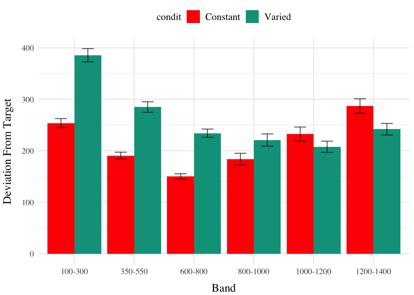
Descriptive summaries testing deviation data are provided in Table 2 and Figure 1. To model differences in accuracy between groups, we used Bayesian mixed effects regression models to the trial level data from the testing phase. The primary model predicted the absolute deviation from the target velocity band (dist) as a function of training condition (condit), target velocity band (band), and their interaction, with random intercepts and slopes for each participant (id).

\[\begin{equation} dist_{ij} = \beta_0 + \beta_1 \cdot condit_{ij} + \beta_2 \cdot band_{ij} + \beta_3 \cdot condit_{ij} \cdot band_{ij} + b_{0i} + b_{1i} \cdot band_{ij} + \epsilon_{ij} \end{equation}\]

datasummary(vx*vb ~ Mean + SD + Histogram, data = testAvg)

datasummary(vx*vb*condit ~ Mean + SD + Histogram, data = testAvg)

result <- test_summary_table(test, "dist","Deviation", mfun = list(mean = mean, median = median, sd = sd))
result$constant |> kbl()
result$varied |> kbl()

Table 2: Testing Deviation - Empirical Summary

(a) Constant Testing - Deviation

Band	Band Type	Mean	Median	Sd
100-300	Extrapolation	254	148	298
350-550	Extrapolation	191	110	229
600-800	Extrapolation	150	84	184
800-1000	Trained	184	106	242
1000-1200	Extrapolation	233	157	282
1200-1400	Extrapolation	287	214	290

(b) Varied Testing - Deviation

Band	Band Type	Mean	Median	Sd
100-300	Extrapolation	386	233	426
350-550	Extrapolation	285	149	340
600-800	Extrapolation	234	144	270
800-1000	Trained	221	149	248
1000-1200	Trained	208	142	226
1200-1400	Trained	242	182	235

test |>  ggplot(aes(x = vb, y = dist,fill=condit)) +
    stat_summary(geom = "bar", position=position_dodge(), fun = mean) +
    stat_summary(geom = "errorbar", position=position_dodge(.9), fun.data = mean_se, width = .4, alpha = .7) + 
  labs(x="Band", y="Deviation From Target")

Figure 1: E1. Deviations from target band during testing without feedback stage.

#options(brms.backend="cmdstanr",mc.cores=4)
modelFile <- paste0(here::here("data/model_cache/"), "e1_dist_Cond_Type_RF_2")
bmtd <- brm(dist ~ condit * bandType + (1|bandInt) + (1|id), 
    data=testE1, file=modelFile,
    iter=5000,chains=4, control = list(adapt_delta = .94, max_treedepth = 13))
                        
#bayestestR::describe_posterior(bmtd)

mted1 <- as.data.frame(describe_posterior(bmtd, centrality = "Mean"))[, c(1,2,4,5,6)]
colnames(mted1) <- c("Term", "Estimate","95% CrI Lower", "95% CrI Upper", "pd")


# r_bandInt_params <- get_variables(bmtd)[grepl("r_bandInt", get_variables(bmtd))]
# posterior_summary(bmtd,variable=r_bandInt_params)
# 
# r_bandInt_params <- get_variables(bmtd)[grepl("r_id:bandInt", get_variables(bmtd))]
# posterior_summary(bmtd,variable=r_bandInt_params)

mted1 |> mutate(across(where(is.numeric), \(x) round(x, 2))) |>
  tibble::remove_rownames() |> 
  mutate(Term = stringr::str_remove(Term, "b_")) |> kable(booktabs = TRUE)
cdted1 <- get_coef_details(bmtd, "conditVaried")
cdted2 <-get_coef_details(bmtd, "bandTypeExtrapolation")
cdted3 <-get_coef_details(bmtd, "conditVaried:bandTypeExtrapolation")

Table 3: E1. Training vs. Extrapolation

Term	Estimate	95% CrI Lower	95% CrI Upper	pd
Intercept	152.55	70.63	229.85	1.0
conditVaried	39.00	-21.10	100.81	0.9
bandTypeExtrapolation	71.51	33.24	109.60	1.0
conditVaried:bandTypeExtrapolation	66.46	32.76	99.36	1.0

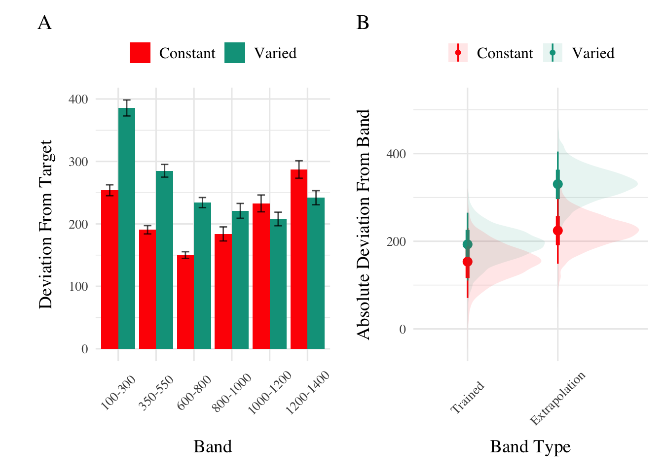
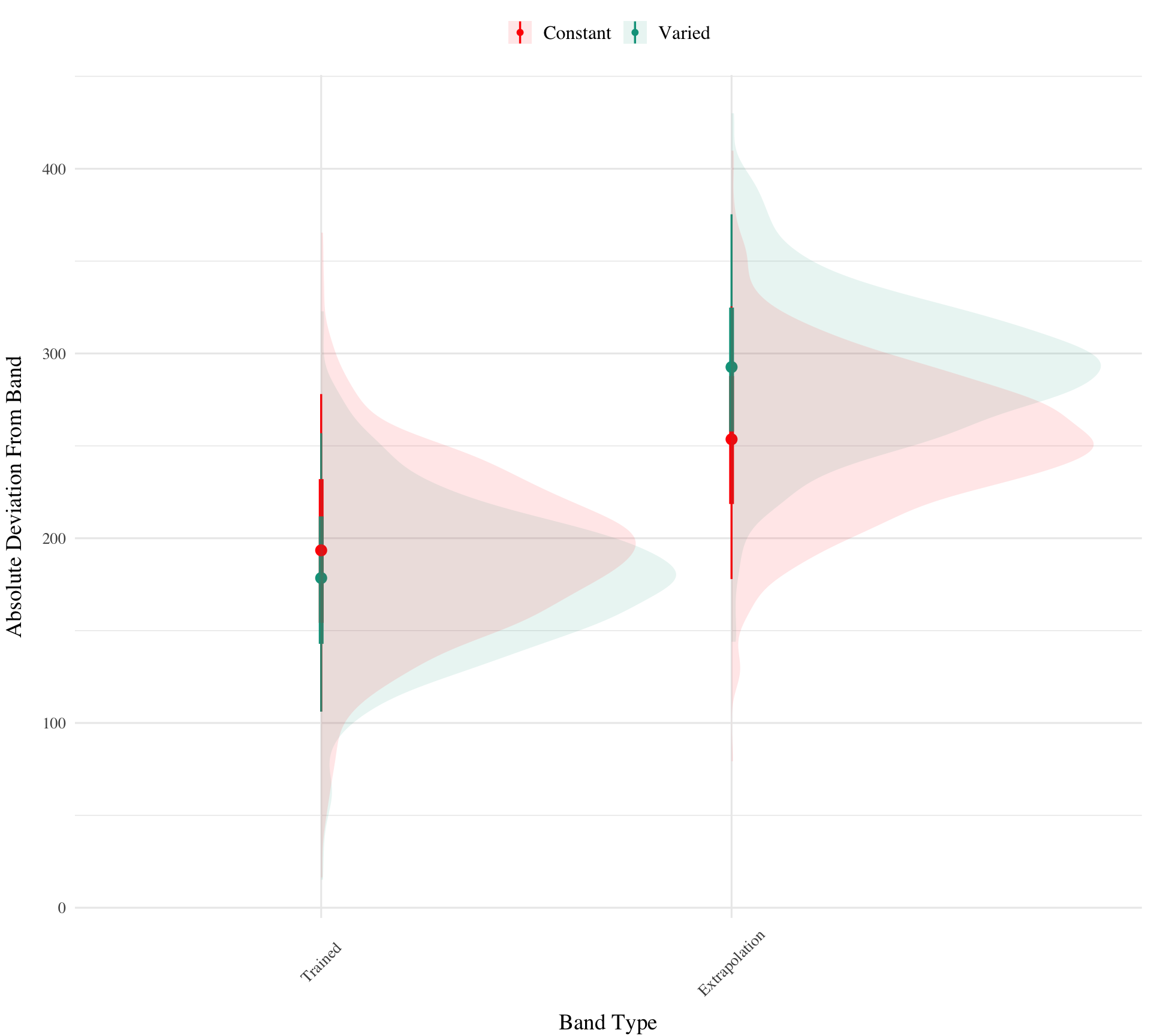
Testing. To compare conditions in the testing stage, we first fit a model predicting deviation from the target band as a function of training condition and band type, with random intercepts for participants and bands. The model is shown in Table 3. The effect of training condition was not reliably different from 0 (β = 39, 95% CrI [-21.1, 100.81]; pd = 89.93%). The extrapolation testing items had a significantly greater deviation than the interpolation band (β = 71.51, 95% CrI [33.24, 109.6]; pd = 99.99%). The interaction between training condition and band type was significant (β = 66.46, 95% CrI [32.76, 99.36]; pd = 99.99%), with the varied group showing a greater deviation than the constant group in the extrapolation bands. See Figure 2.

pe1td <- testE1 |>  ggplot(aes(x = vb, y = dist,fill=condit)) +
    stat_summary(geom = "bar", position=position_dodge(), fun = mean) +
    stat_summary(geom = "errorbar", position=position_dodge(.9), fun.data = mean_se, width = .4, alpha = .7) + 
  theme(legend.title=element_blank(),axis.text.x = element_text(angle = 45, hjust = 0.5, vjust = 0.5)) +
  labs(x="Band", y="Deviation From Target")

condEffects <- function(m,xvar){
  m |> ggplot(aes(x = {{xvar}}, y = .value, color = condit, fill = condit)) + 
  stat_dist_pointinterval() + 
  stat_halfeye(alpha=.1, height=.5) +
  theme(legend.title=element_blank(),axis.text.x = element_text(angle = 45, hjust = 0.5, vjust = 0.5)) 
  
}

pe1ce <- bmtd |> emmeans( ~condit + bandType) |>
  gather_emmeans_draws() |>
 condEffects(bandType) + labs(y="Absolute Deviation From Band", x="Band Type")

Loading required namespace: rstanarm

(pe1td + pe1ce) + plot_annotation(tag_levels= 'A')

Figure 2: E1. Deviations from target band during testing without feedback stage.

#contrasts(test$condit) 
#contrasts(test$vb)
modelName <- "e1_testDistBand_RF_5K"
e1_distBMM <- brm(dist ~ condit * bandInt + (1 + bandInt|id),
                      data=test,file=paste0(here::here("data/model_cache",modelName)),
                      iter=5000,chains=4)
GetModelStats(e1_distBMM) |> kable(escape=F,booktabs=T,caption="Model Coefficients")
e1_distBMM |> 
  emmeans("condit",by="bandInt",at=list(bandInt=c(100,350,600,800,1000,1200)),
          epred = TRUE, re_formula = NA) |> 
  pairs() |> gather_emmeans_draws()  |> 
   summarize(median_qi(.value),pd=sum(.value>0)/n()) |>
   select(contrast,Band=bandInt,value=y,lower=ymin,upper=ymax,pd) |> 
   mutate(across(where(is.numeric), \(x) round(x, 2)),
          pd=ifelse(value<0,1-pd,pd)) |>
   kbl(caption="Contrasts")
coef_details <- get_coef_details(e1_distBMM, "conditVaried")

Table 4: Experiment 1. Bayesian Mixed Model predicting absolute deviation as a function of condition (Constant vs. Varied) and Velocity Band

Model Coefficients

Term	Estimate	95% CrI Lower	95% CrI Upper	pd
Intercept	205.09	136.86	274.06	1.00
conditVaried	157.44	60.53	254.90	1.00
Band	0.01	-0.07	0.08	0.57
condit*Band	-0.16	-0.26	-0.06	1.00

Contrasts

contrast	Band	value	lower	upper	pd
Constant - Varied	100	-141.49	-229.19	-53.83	1.00
Constant - Varied	350	-101.79	-165.62	-36.32	1.00
Constant - Varied	600	-62.02	-106.21	-14.77	1.00
Constant - Varied	800	-30.11	-65.08	6.98	0.94
Constant - Varied	1000	2.05	-33.46	38.41	0.54
Constant - Varied	1200	33.96	-11.94	81.01	0.92

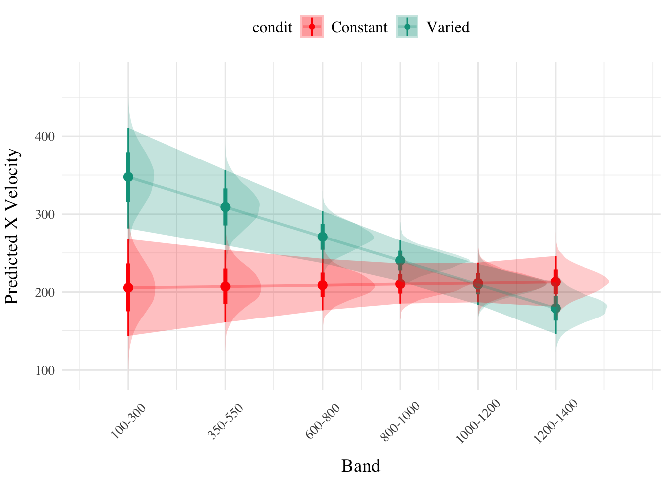
The model predicting absolute deviation (dist) showed clear effects of both training condition and target velocity band (Table X). Overall, the varied training group showed a larger deviation relative to the constant training group (β = 157.44, 95% CI [60.53, 254.9]). Deviation also depended on target velocity band, with lower bands showing less deviation. See Table 3 for full model output.

condEffects <- function(m){
  m |> ggplot(aes(x = bandInt, y = .value, color = condit, fill = condit)) + 
  stat_dist_pointinterval() + stat_halfeye(alpha=.2) +
  stat_lineribbon(alpha = .25, size = 1, .width = c(.95)) +
  theme(axis.text.x = element_text(angle = 45, hjust = 0.5, vjust = 0.5)) +
  ylab("Predicted X Velocity") + xlab("Band")
}

e1_distBMM |> emmeans( ~condit + bandInt, 
                       at = list(bandInt = c(100, 350, 600, 800, 1000, 1200))) |>
  gather_emmeans_draws() |>
 condEffects()+
  scale_x_continuous(breaks = c(100, 350, 600, 800, 1000, 1200), 
                     labels = levels(test$vb), 
                     limits = c(0, 1400)) 

Figure 3: E1. Conditioinal Effect of Training Condition and Band. Ribbon indicated 95% Credible Intervals.

Discrimination between bands

In addition to accuracy/deviation, we also assessed the ability of participants to reliably discriminate between the velocity bands (i.e. responding differently when prompted for band 600-800 than when prompted for band 150-350). Table 5 shows descriptive statistics of this measure, and Figure 1 visualizes the full distributions of throws for each combination of condition and velocity band. To quantify discrimination, we again fit Bayesian Mixed Models as above, but this time the dependent variable was the raw x velocity generated by participants on each testing trial.

\[\begin{equation} vx_{ij} = \beta_0 + \beta_1 \cdot condit_{ij} + \beta_2 \cdot bandInt_{ij} + \beta_3 \cdot condit_{ij} \cdot bandInt_{ij} + b_{0i} + b_{1i} \cdot bandInt_{ij} + \epsilon_{ij} \end{equation}\]

test %>% group_by(id,vb,condit) |> plot_distByCondit()

Figure 4: E1 testing x velocities. Translucent bands with dash lines indicate the correct range for each velocity band.

result <- test_summary_table(test, "vx","X Velocity", mfun = list(mean = mean, median = median, sd = sd))
result$constant |> kable()
result$varied |> kable()

Table 5: Testing vx - Empirical Summary

(a) Constant Testing - vx

Band	Band Type	Mean	Median	Sd
100-300	Extrapolation	524	448	327
350-550	Extrapolation	659	624	303
600-800	Extrapolation	770	724	300
800-1000	Trained	1001	940	357
1000-1200	Extrapolation	1167	1104	430
1200-1400	Extrapolation	1283	1225	483

(b) Varied Testing - vx

Band	Band Type	Mean	Median	Sd
100-300	Extrapolation	664	533	448
350-550	Extrapolation	768	677	402
600-800	Extrapolation	876	813	390
800-1000	Trained	1064	1029	370
1000-1200	Trained	1180	1179	372
1200-1400	Trained	1265	1249	412

e1_vxBMM <- brm(vx ~ condit * bandInt + (1 + bandInt|id),
                        data=test,file=paste0(here::here("data/model_cache", "e1_testVxBand_RF_5k")),
                        iter=5000,chains=4,silent=0,
                        control=list(adapt_delta=0.94, max_treedepth=13))
GetModelStats(e1_vxBMM ) |> kable(escape=F,booktabs=T, caption="Fit to all 6 bands")
cd1 <- get_coef_details(e1_vxBMM, "conditVaried")
sc1 <- get_coef_details(e1_vxBMM, "bandInt")
intCoef1 <- get_coef_details(e1_vxBMM, "conditVaried:bandInt")


modelName <- "e1_extrap_testVxBand"
e1_extrap_VxBMM <- brm(vx ~ condit * bandInt + (1 + bandInt|id),
                  data=test |>
                    filter(expMode=="test-Nf"),file=paste0(here::here("data/model_cache",modelName)),
                  iter=5000,chains=4)
GetModelStats(e1_extrap_VxBMM ) |> kable(escape=F,booktabs=T, caption="Fit to 3 extrapolation bands")
sc2 <- get_coef_details(e1_extrap_VxBMM, "bandInt")
intCoef2 <- get_coef_details(e1_extrap_VxBMM, "conditVaried:bandInt")

Table 6: Experiment 1. Bayesian Mixed Model Predicting Vx as a function of condition (Constant vs. Varied) and Velocity Band

(a) Model fit to all 6 bands

Term	Estimate	95% CrI Lower	95% CrI Upper	pd
Intercept	408.55	327.00	490.61	1.00
conditVaried	164.05	45.50	278.85	1.00
Band	0.71	0.62	0.80	1.00
condit*Band	-0.14	-0.26	-0.01	0.98

(b) Model fit to 3 extrapolation bands

Term	Estimate	95% CrI Lower	95% CrI Upper	pd
Intercept	497.49	431.26	566.17	1.00
conditVaried	124.79	26.61	224.75	0.99
Band	0.49	0.42	0.56	1.00
condit*Band	-0.06	-0.16	0.04	0.88

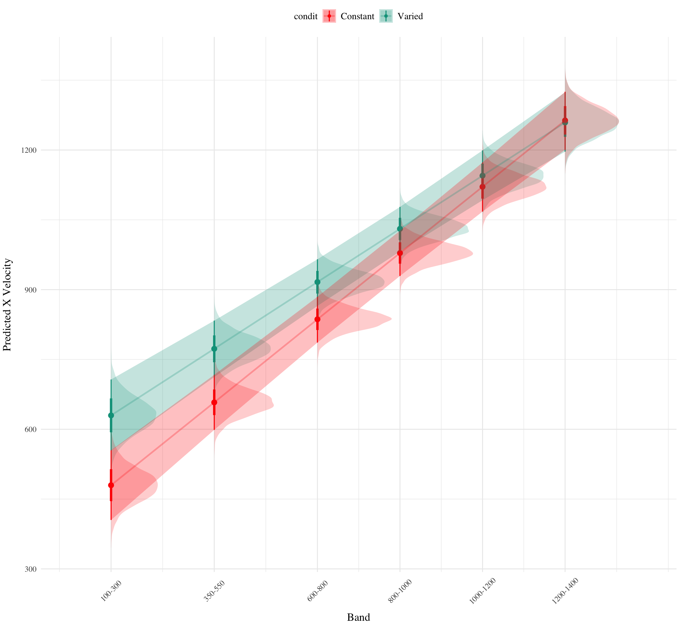
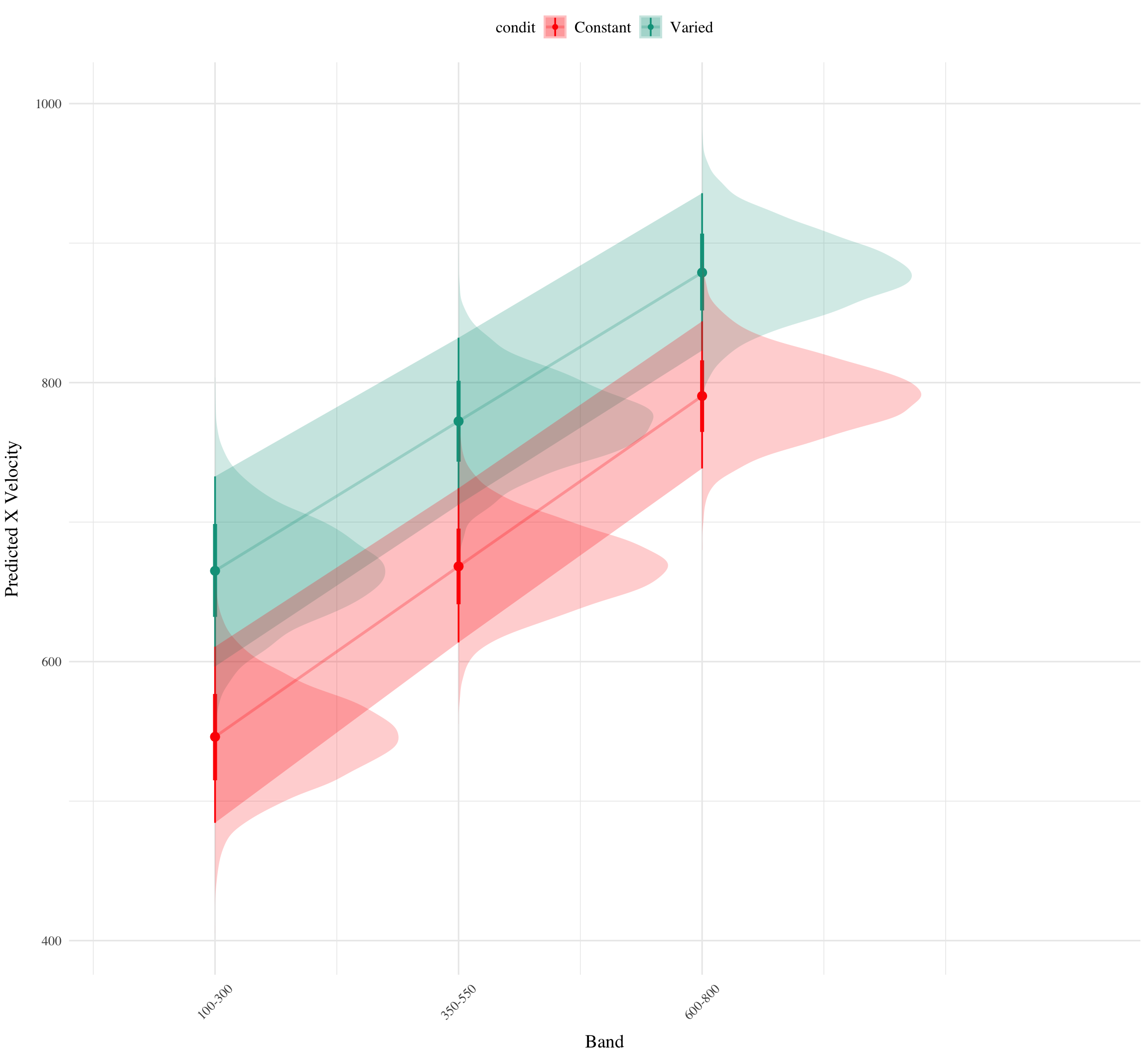
See Table 6 for the full model results. The estimated coefficient for training condition (β = 164.05, 95% CrI [45.5, 278.85]) suggests that the varied group tends to produce harder throws than the constant group, but is not in and of itself useful for assessing discrimination. Most relevant to the issue of discrimination is the slope on Velocity Band (β = 0.71, 95% CrI [0.62, 0.8]). Although the median slope does fall underneath the ideal of value of 1, the fact that the 95% credible interval does not contain 0 provides strong evidence that participants exhibited some discrimination between bands. The estimate for the interaction between slope and condition (β = -0.14, 95% CrI [-0.26, -0.01]), suggests that the discrimination was somewhat modulated by training condition, with the varied participants showing less sensitivity between bands than the constant condition. This difference is depicted visually in Figure 5. Table 7 shows the average slope coefficients for varied and constant participants separately for each quartile. The constant participant participants appear to have larger slopes across quartiles, but the difference between conditions may be less pronounced for the top quartiles of subjects who show the strongest discrimination. Figure Figure 6 shows the distributions of slope values for each participant, and the compares the probability density of slope coefficients between training conditions. Figure 7

The second model, which focused solely on extrapolation bands, revealed similar patterns. The Velocity Band term (β = 0.49, 95% CrI [0.42, 0.56]) still demonstrates a high degree of discrimination ability. However, the posterior distribution for interaction term (β = -0.06, 95% CrI [-0.16, 0.04] ) does across over 0, suggesting that the evidence for decreased discrimination ability for the varied participants is not as strong when considering only the three extrapolation bands.

e1_vxBMM |> emmeans( ~condit + bandInt, 
                       at = list(bandInt = c(100, 350, 600, 800, 1000, 1200))) |>
  gather_emmeans_draws() |> 
  condEffects() +
  scale_x_continuous(breaks = c(100, 350, 600, 800, 1000, 1200), 
                     labels = levels(test$vb), 
                     limits = c(0, 1400))

e1_extrap_VxBMM |> emmeans( ~condit + bandInt, 
                       at = list(bandInt = c(100, 350, 600))) |>
  gather_emmeans_draws() |>
  condEffects() +
  scale_x_continuous(breaks = c(100, 350, 600), 
                     labels = levels(test$vb)[1:3], 
                     limits = c(0, 1000)) 

(a) Model fit to all 6 bands

(b) Model fit to only 3 extrapolation bands

Figure 5: Conditional effect of training condition and Band. Ribbons indicate 95% HDI. The steepness of the lines serves as an indicator of how well participants discriminated between velocity bands.

new_data_grid=map_dfr(1, ~data.frame(unique(test[,c("id","condit","bandInt")]))) |> 
  dplyr::arrange(id,bandInt) |> 
  mutate(condit_dummy = ifelse(condit == "Varied", 1, 0)) 

indv_coefs <- as_tibble(coef(e1_vxBMM)$id, rownames="id")|> 
  select(id, starts_with("Est")) |>
  left_join(e1Sbjs, by=join_by(id) ) 


fixed_effects <- e1_vxBMM |> 
  spread_draws(`^b_.*`,regex=TRUE) |> arrange(.chain,.draw,.iteration)


random_effects <- e1_vxBMM |> 
  gather_draws(`^r_id.*$`, regex = TRUE, ndraws = 500) |> 
  separate(.variable, into = c("effect", "id", "term"), sep = "\\[|,|\\]") |> 
  mutate(id = factor(id,levels=levels(test$id))) |> 
  pivot_wider(names_from = term, values_from = .value) |> arrange(id,.chain,.draw,.iteration)

Warning: Expected 3 pieces. Additional pieces discarded in 156000 rows [1, 2, 3, 4, 5,
6, 7, 8, 9, 10, 11, 12, 13, 14, 15, 16, 17, 18, 19, 20, ...].

 indvDraws <- left_join(random_effects, fixed_effects, by = join_by(".chain", ".iteration", ".draw")) |> 
  rename(bandInt_RF = bandInt,RF_Intercept=Intercept) |>
  right_join(new_data_grid, by = join_by("id")) |> 
  mutate(
    Slope = bandInt_RF+b_bandInt,
    Intercept= RF_Intercept + b_Intercept,
    estimate = (b_Intercept + RF_Intercept) + (bandInt*(b_bandInt+bandInt_RF)) + (bandInt * condit_dummy) * `b_conditVaried:bandInt`,
    SlopeInt = Slope + (`b_conditVaried:bandInt`*condit_dummy)
  ) 

Warning in right_join(rename(left_join(random_effects, fixed_effects, by = join_by(".chain", : Detected an unexpected many-to-many relationship between `x` and `y`.
ℹ Row 1 of `x` matches multiple rows in `y`.
ℹ Row 1 of `y` matches multiple rows in `x`.
ℹ If a many-to-many relationship is expected, set `relationship =
  "many-to-many"` to silence this warning.

  indvSlopes <- indvDraws |> group_by(id) |> median_qi(Slope,SlopeInt, Intercept,b_Intercept,b_bandInt) |>
  left_join(e1Sbjs, by=join_by(id)) |> group_by(condit) |>
    select(id,condit,Intercept,b_Intercept,starts_with("Slope"),b_bandInt, n) |>
  mutate(rankSlope=rank(Slope)) |> arrange(rankSlope)   |> ungroup()
 
  
  indvSlopes |> mutate(Condition=condit) |>  group_by(Condition) |> 
    reframe(enframe(quantile(SlopeInt, c(0.0,0.25, 0.5, 0.75,1)), "quantile", "SlopeInt")) |> 
  pivot_wider(names_from=quantile,values_from=SlopeInt,names_prefix="Q_") |>
  group_by(Condition) |>
  summarise(across(starts_with("Q"), list(mean = mean))) |> kbl()

Table 7: Slope coefficients by quartile, per condition

Condition	Q_0%_mean	Q_25%_mean	Q_50%_mean	Q_75%_mean	Q_100%_mean
Constant	-0.1065285	0.4813997	0.6901252	0.9368777	1.398519
Varied	-0.2039670	0.2703687	0.5939692	0.8950950	1.288174

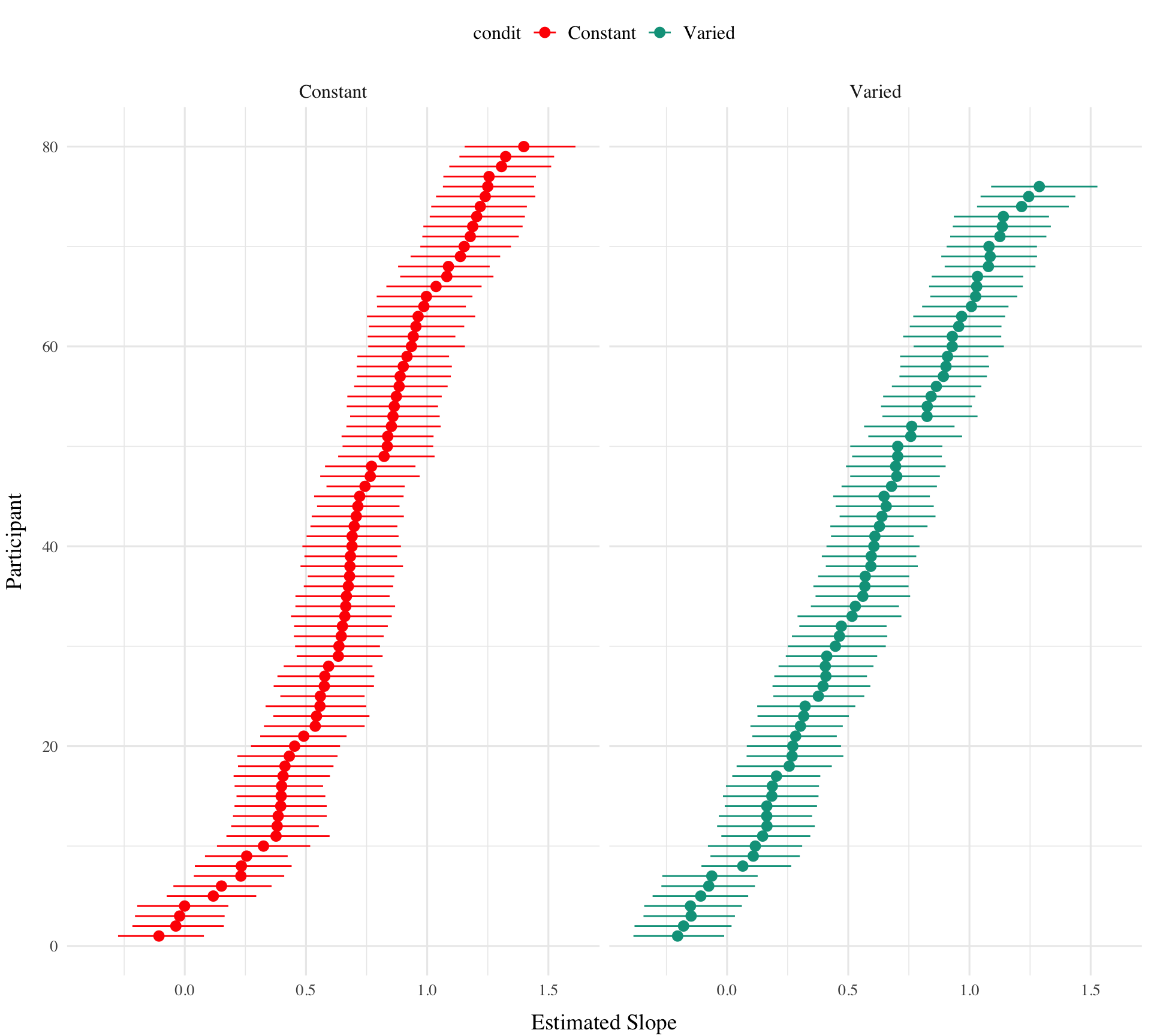
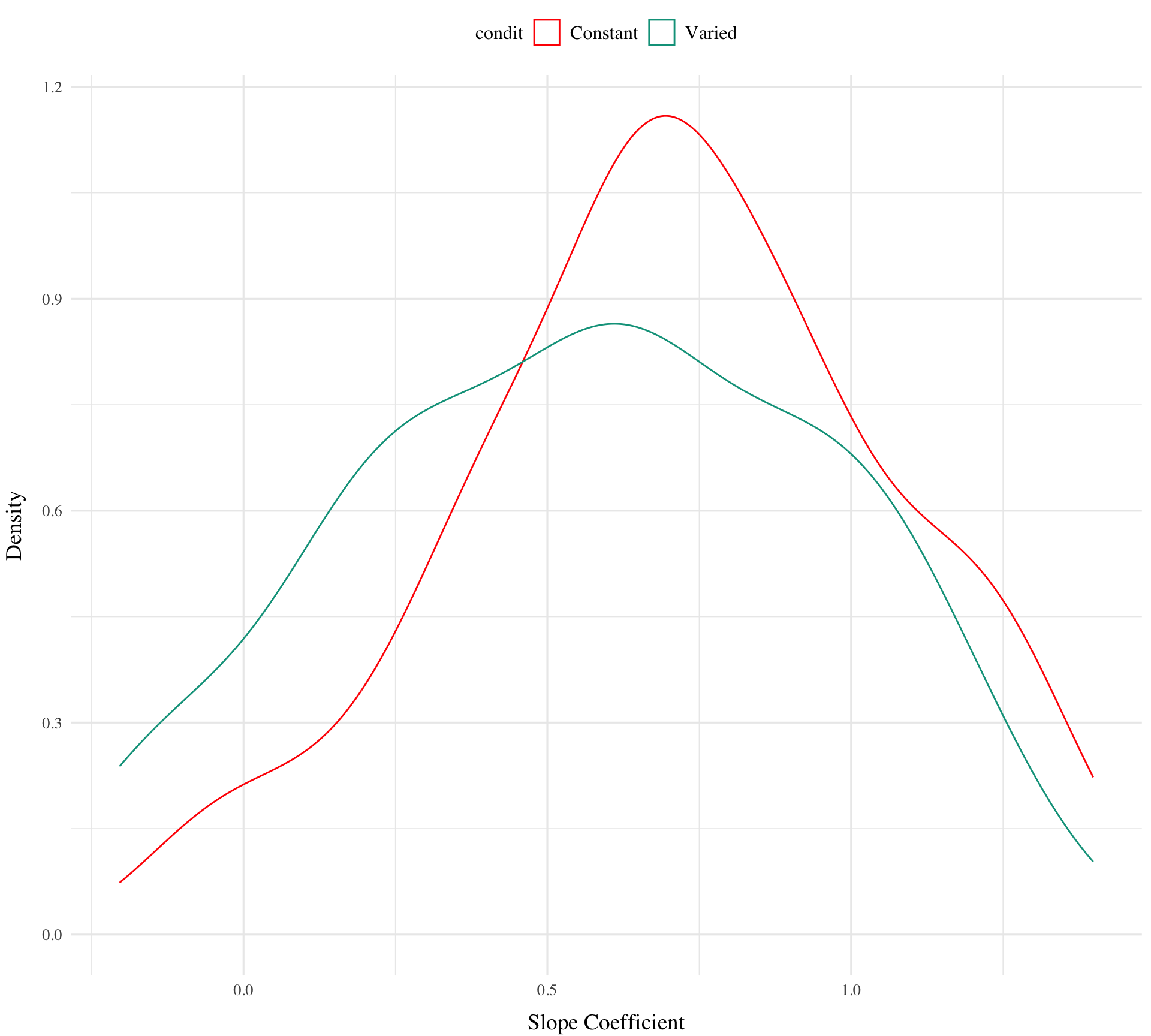
Figure 6 shows the distributions of estimated slopes relating velocity band to x velocity for each participant, ordered from lowest to highest within condition. Slope values are lower overall for varied training compared to constant training. Figure Xb plots the density of these slopes for each condition. The distribution for varied training has more mass at lower values than the constant training distribution. Both figures illustrate the model’s estimate that varied training resulted in less discrimination between velocity bands, evidenced by lower slopes on average.

  indvSlopes |> ggplot(aes(y=rankSlope, x=SlopeInt,fill=condit,color=condit)) + 
  geom_pointrange(aes(xmin=SlopeInt.lower , xmax=SlopeInt.upper)) + 
  labs(x="Estimated Slope", y="Participant")  + facet_wrap(~condit)

   ggplot(indvSlopes, aes(x = SlopeInt, color = condit)) + 
  geom_density() + labs(x="Slope Coefficient",y="Density")

(a) Slope estimates by participant - ordered from lowest to highest within each condition.

(b) Destiny of slope coefficients by training group

Figure 6: Slope distributions between condition

nSbj <- 3
indvDraws  |> indv_model_plot(indvSlopes, testAvg, SlopeInt,rank_variable=Slope,n_sbj=nSbj,"max")
indvDraws |> indv_model_plot(indvSlopes, testAvg,SlopeInt, rank_variable=Slope,n_sbj=nSbj,"min")

(a) subset with largest slopes

(b) subset with smallest slopes

Figure 7: Subset of Varied and Constant Participants with the smallest and largest estimated slope values. Red lines represent the best fitting line for each participant, gray lines are 200 random samples from the posterior distribution. Colored points and intervals at each band represent the empirical median and 95% HDI.

control for training end performance

testE1 |> group_by(id,condit) |> pivot_longer(c("dist","train_end"),names_to="var",values_to="value") |> 
  ggplot(aes(x=var,y=value, fill=condit)) + stat_bar + facet_wrap(~var)

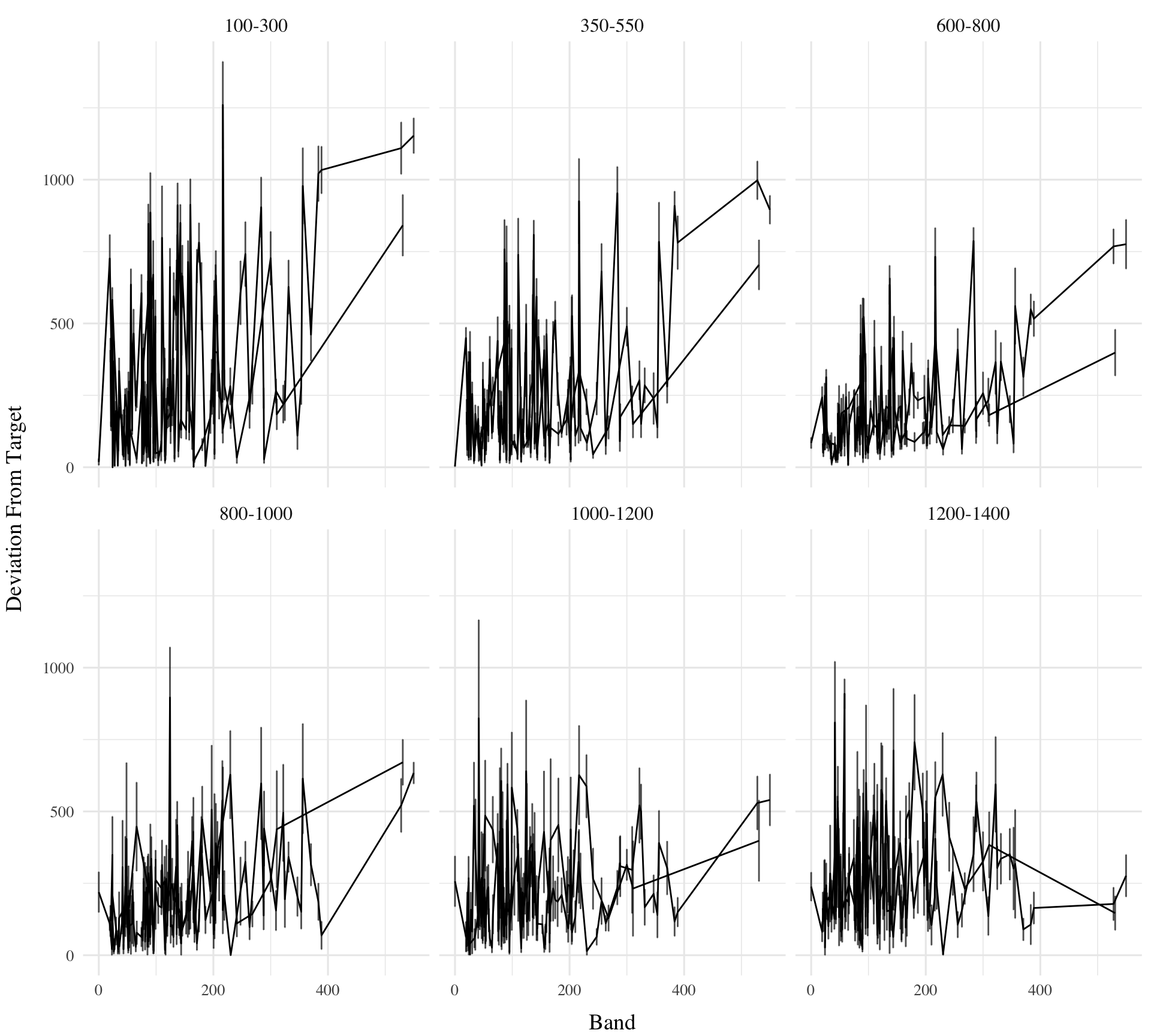
testE1 |> ggplot(aes(x=train_end,y=dist,fill=condit)) + 
  stat_summary(geom = "line", position=position_dodge(), fun = mean) +
    stat_summary(geom = "errorbar", position=position_dodge(.9), fun.data = mean_se, width = .4, alpha = .7) + 
    facet_wrap(~vb) +
  labs(x="Band", y="Deviation From Target")

Warning: Width not defined
ℹ Set with `position_dodge(width = ...)`

Warning: `position_dodge()` requires non-overlapping x intervals.
`position_dodge()` requires non-overlapping x intervals.
`position_dodge()` requires non-overlapping x intervals.
`position_dodge()` requires non-overlapping x intervals.
`position_dodge()` requires non-overlapping x intervals.
`position_dodge()` requires non-overlapping x intervals.

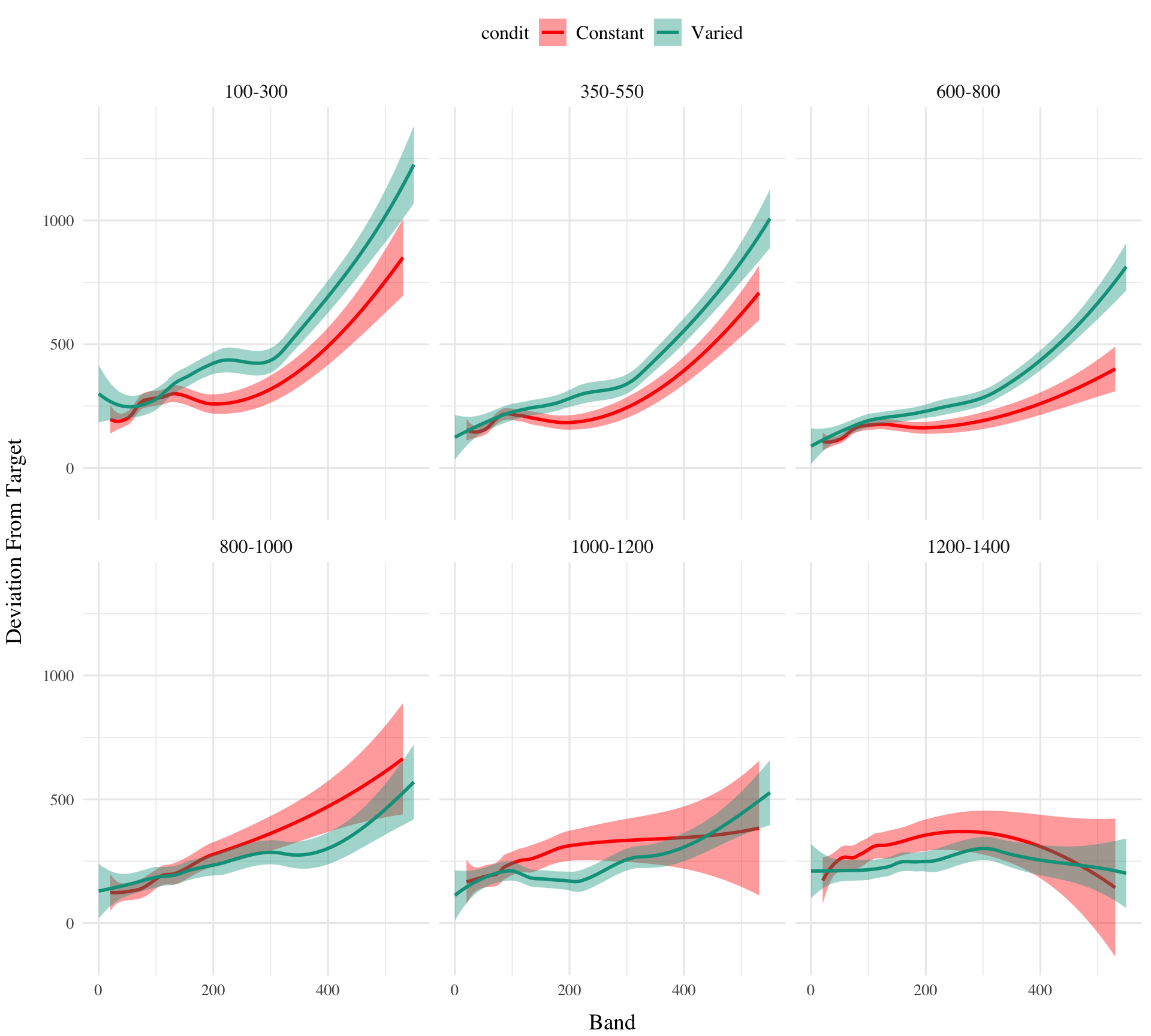
testE1 |> ggplot(aes(x=train_end,y=dist,fill=condit,col=condit)) + 
  #geom_point() +
  geom_smooth(method="loess") +
    facet_wrap(~vb) +
  labs(x="Band", y="Deviation From Target")

`geom_smooth()` using formula = 'y ~ x'

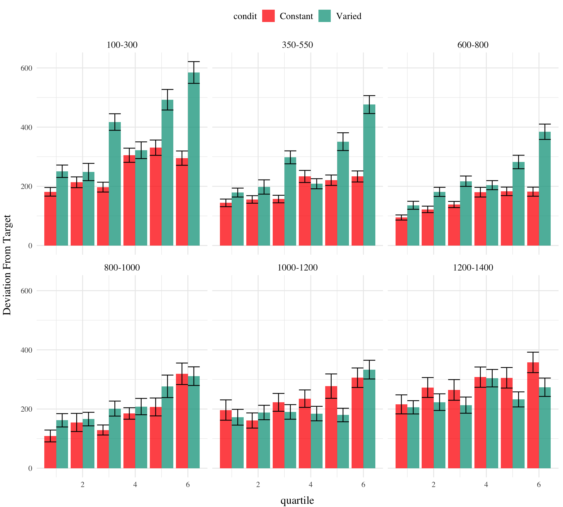
# create quartiles for train_end
testE1 |> group_by(condit,vb) |> 
  mutate(train_end_q = ntile(train_end,6)) |> 
  ggplot(aes(x=train_end_q,y=dist,fill=condit)) + 
 stat_bar + 
    facet_wrap(~vb) +
  labs(x="quartile", y="Deviation From Target")

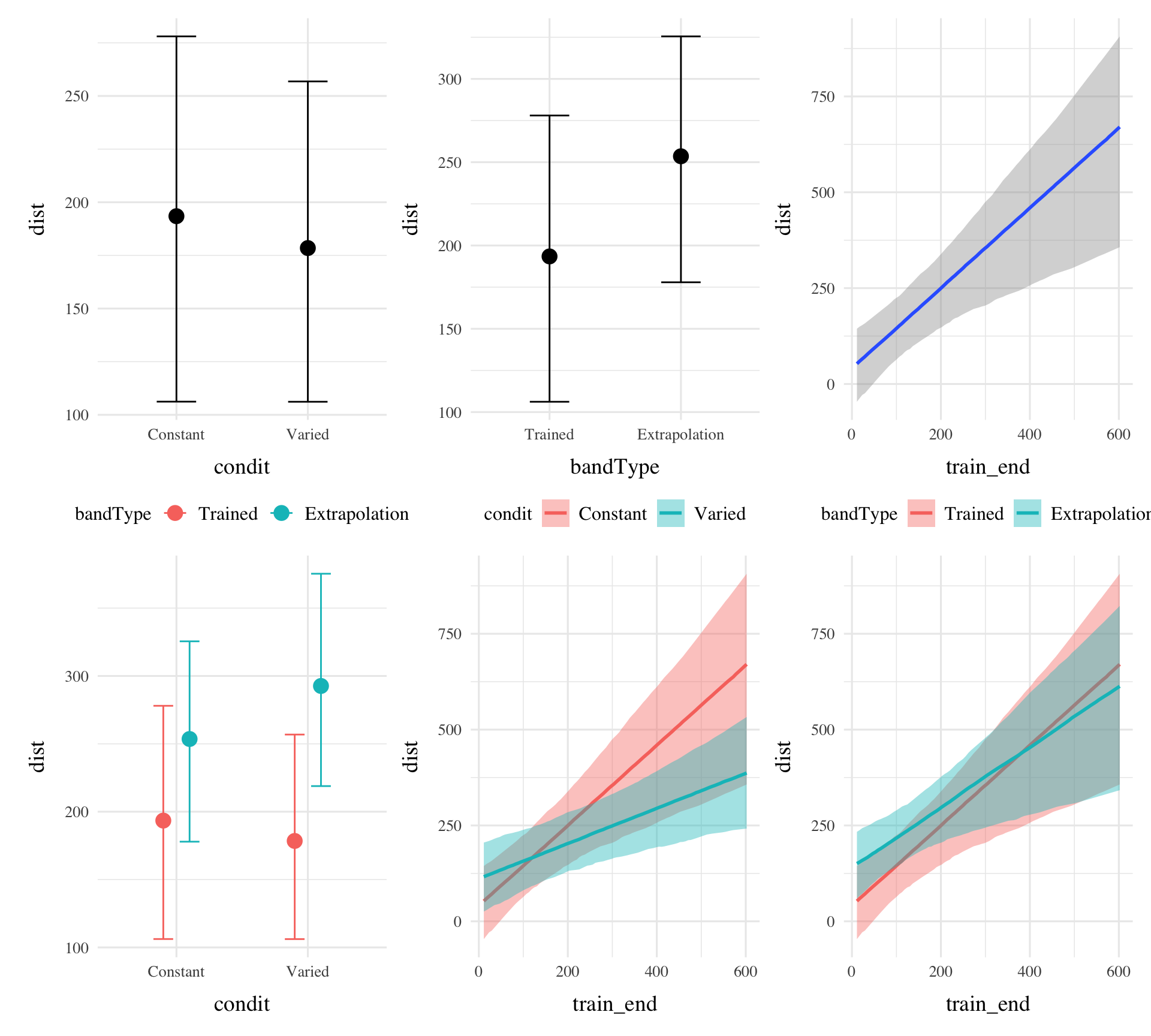
bmtd3 <- brm(dist ~ condit * bandType * train_end + (1|bandInt) + (1|id), 
    data=testE1, 
    file=paste0(here::here("data/model_cache","e1_trainEnd_BT_RF2")),
    iter=1000,chains=2, control = list(adapt_delta = .92, max_treedepth = 11))
summary(bmtd3)

 Family: gaussian 
  Links: mu = identity; sigma = identity 
Formula: dist ~ condit * bandType * train_end + (1 | bandInt) + (1 | id) 
   Data: testE1 (Number of observations: 9491) 
  Draws: 2 chains, each with iter = 1000; warmup = 500; thin = 1;
         total post-warmup draws = 1000

Group-Level Effects: 
~bandInt (Number of levels: 6) 
              Estimate Est.Error l-95% CI u-95% CI Rhat Bulk_ESS Tail_ESS
sd(Intercept)    73.85     31.99    35.91   157.68 1.00      215      429

~id (Number of levels: 156) 
              Estimate Est.Error l-95% CI u-95% CI Rhat Bulk_ESS Tail_ESS
sd(Intercept)   140.36      8.62   125.43   159.07 1.03      111      142

Population-Level Effects: 
                                             Estimate Est.Error l-95% CI
Intercept                                       43.41     49.99   -62.85
conditVaried                                    67.01     49.92   -32.25
bandTypeExtrapolation                           97.92     27.14    45.56
train_end                                        1.02      0.28     0.45
conditVaried:bandTypeExtrapolation             -76.93     27.48  -132.46
conditVaried:train_end                          -0.56      0.31    -1.11
bandTypeExtrapolation:train_end                 -0.26      0.17    -0.58
conditVaried:bandTypeExtrapolation:train_end     0.89      0.18     0.52
                                             u-95% CI Rhat Bulk_ESS Tail_ESS
Intercept                                      136.23 1.01      140      255
conditVaried                                   154.69 1.05       71      147
bandTypeExtrapolation                          151.52 1.00      290      382
train_end                                        1.51 1.01      115      221
conditVaried:bandTypeExtrapolation             -22.04 1.00      273      487
conditVaried:train_end                           0.11 1.03       87      205
bandTypeExtrapolation:train_end                  0.09 1.01      205      310
conditVaried:bandTypeExtrapolation:train_end     1.24 1.01      207      432

Family Specific Parameters: 
      Estimate Est.Error l-95% CI u-95% CI Rhat Bulk_ESS Tail_ESS
sigma   240.85      1.82   237.19   244.52 1.00     1029      512

Draws were sampled using sample(hmc). For each parameter, Bulk_ESS
and Tail_ESS are effective sample size measures, and Rhat is the potential
scale reduction factor on split chains (at convergence, Rhat = 1).

bayestestR::describe_posterior(bmtd3)

Summary of Posterior Distribution

Parameter                                    | Median |            95% CI |     pd |            ROPE | % in ROPE |  Rhat |    ESS
---------------------------------------------------------------------------------------------------------------------------------
(Intercept)                                  |  41.58 | [ -62.85, 136.23] | 82.20% | [-29.55, 29.55] |    33.16% | 1.014 | 142.00
conditVaried                                 |  69.52 | [ -32.25, 154.69] | 90.30% | [-29.55, 29.55] |    18.84% | 1.046 |  70.00
bandTypeExtrapolation                        |  97.03 | [  45.56, 151.52] |   100% | [-29.55, 29.55] |        0% | 1.000 | 280.00
train_end                                    |   1.04 | [   0.45,   1.51] | 99.90% | [-29.55, 29.55] |      100% | 1.010 | 108.00
conditVaried:bandTypeExtrapolation           | -76.11 | [-132.46, -22.04] | 99.90% | [-29.55, 29.55] |     2.00% | 1.000 | 268.00
conditVaried:train_end                       |  -0.57 | [  -1.11,   0.11] | 95.10% | [-29.55, 29.55] |      100% | 1.029 |  84.00
bandTypeExtrapolation:train_end              |  -0.27 | [  -0.58,   0.09] | 92.00% | [-29.55, 29.55] |      100% | 1.006 | 204.00
conditVaried:bandTypeExtrapolation:train_end |   0.89 | [   0.52,   1.24] |   100% | [-29.55, 29.55] |      100% | 1.005 | 206.00

condEffects <- function(m,xvar){
  m |> ggplot(aes(x = {{xvar}}, y = .value, color = condit, fill = condit)) + 
  stat_dist_pointinterval() + 
  stat_halfeye(alpha=.1, height=.5) +
  theme(legend.title=element_blank(),axis.text.x = element_text(angle = 45, hjust = 0.5, vjust = 0.5)) 
  
}

 bmtd3 |> emmeans( ~condit * bandType * train_end) |>
  gather_emmeans_draws() |>
 condEffects(bandType) + labs(y="Absolute Deviation From Band", x="Band Type")

ce_bmtd3 <- plot(conditional_effects(bmtd3),points=FALSE,plot=FALSE)
wrap_plots(ce_bmtd3)

E1 Results Discussion

NEEDS TO BE WRITTEN

References

Bürkner, P.-C. (2017). Brms: An R Package for Bayesian Multilevel Models Using Stan. Journal of Statistical Software, 80, 1–28. https://doi.org/10.18637/jss.v080.i01

Makowski, D., Ben-Shachar, M. S., & Lüdecke, D. (2019). bayestestR: Describing Effects and their Uncertainty, Existence and Significance within the Bayesian Framework. Journal of Open Source Software, 4(40), 1541. https://doi.org/10.21105/joss.01541

Team, R. C. (2020). R: A Language and Environment for Statistical Computing. R: A Language and Environment for Statistical Computing.