Mermaid with R + consort

#lapply(c('tidyverse','data.table','igraph','ggraph','kableExtra'),library,character.only=TRUE))
pacman::p_load(tidyverse,data.table,igraph,ggraph,kableExtra,DiagrammeR,png,consort,data.table) 

flowchart LR
    data1(Varied Training<br/>800-1000<br/>1000-1200<br/>1200-1400)
    data2(Constant Training<br/>800-1000)
    Test1(Testing - No Feedback<br/>100-300<br/>350-550<br/>600-800)
    Test2(Test From Train<br/>800-1000<br/>1000-1200<br/>1200-1400)
    Test3(Testing - Feedback<br/>100-300<br/>350-550<br/>600-800)

    data1 --> Test1
    data2 --> Test1
    Test1 --> Test2
    Test2 --> Test3
    
%% https://quarto.org/docs/authoring/diagrams.html

Mean Vx over training blocks

Figure 1: This is a simple graphviz graph.

Figure 2: This is a simple graphviz graph.

subgraph

test

test2

test3

test4

Nest Cluster - GraphViz

test5

test6

test7

test8

grViz('digraph threevar {
      rankdir=LR;
      size="8,4";
      node [fontsize=14 shape=box];
      edge [fontsize=10];
      center=1;
      {rank=min k }
      {rank=same X1 X2 X3 }
      {rank=max z1 z2 z3 }
      z1 [shape=circle label="d1"];
      z2 [shape=circle label="d2"];
      z3 [shape=circle label="d3"];
      k [label="?" shape="ellipse"];
      k -> X1 [label="n@_{S}"];
      k -> X2 [label="θ@^{(h)}"];
      k -> X3 [label="?3"];
      z1 -> X1;
      z2 -> X2;
      z3 -> X3;
    }
      ')

grViz("digraph dot {
      graph [style = filled, fillcolor = white]
      
      node [shape = circle,
            style = filled, fillcolor = white,
            fixedsize = true, width = 0.5, height = 0.5,
            fontname = 'Times-italic']
        c
        d
      node [shape = doublecircle,
            style = filled, fillcolor = white,
            fixedsize = true, width = 0.5, height = 0.5,
            fontname = 'Times-italic']
        thetah [label = 'θ@^{(h)}']
        thetaf [label = 'θ@^{(f)}']
      node [shape = square,
            style = filled, fillcolor = grey,
            fixedsize = true, width=0.5, height=0.5,
            fontname = 'Times-italic']
        h
        f
        ns [label = 'n@_{S}']
        nn [label = 'n@_{N}']
      
      edge [color = black]
        c -> thetah -> h
        d -> thetaf -> f
        c -> thetaf
        d -> thetah
        ns -> h
        nn -> f
      {rank = max; ns; nn}
      }")

grViz("digraph dot {
      graph [style = filled, fillcolor = white,
             rankdir = LR,
             newrank = true]
      
      node [shape = circle,
            style = filled, fillcolor = white,
            fixedsize = true, width = 0.5, height = 0.5,
            fontname = 'Times-italic']
        p [fillcolor = gray]
        gamma [label = 'γ']
        omega [label = 'ω', shape = doublecircle]
        beta [label = 'β']
      subgraph cluster_out{
        fontsize = 8
        label = <<I>j</I>:試行>
        labelloc = b
        labeljust = r
        subgraph cluster_in{
          fontsize = 8
          label = <<I>k</I>:回数>
          labelloc = b
          labeljust = r
          thetajk [label = '&theta;@_{jk}', shape = doublecircle]
          djk [label = 'd@_{jk}', shape = square, fillcolor = gray]
        }}
      edge [color=black]
        p -> omega -> thetajk -> djk
        gamma -> omega
        beta -> thetajk 
      {rank = same; gamma; omega}
      {rank = same; beta; thetajk}
      }")

grViz('
digraph G {
    fontname="Helvetica,Arial,sans-serif"
    node [fontname="Helvetica,Arial,sans-serif"]
    edge [fontname="Helvetica,Arial,sans-serif"]

    subgraph cluster_0 {
        style=filled;
        color=lightgrey;
        node [style=filled,color=white];
        a0 -> a1 -> a2 -> a3;
        label = "process #1";
    }

    subgraph cluster_1 {
        node [style=filled];
        b0 -> b1 -> b2 -> b3;
        label = "process #2";
        color=blue
    }
    start -> a0;
    start -> b0;
    a1 -> b3;
    b2 -> a3;
    a3 -> a0;
    a3 -> end;
    b3 -> end;

    start [shape=Mdiamond];
    end [shape=Msquare];
}')

#https://graphviz.org/Gallery/directed/neural-network.html

grViz('digraph G {
  fontname="Helvetica,Arial,sans-serif"
  node [fontname="Helvetica,Arial,sans-serif"]
  edge [fontname="Helvetica,Arial,sans-serif"]
  concentrate=True;
  rankdir=TB;
  node [shape=record];
  140087530674552 [label="title: InputLayer\n|{input:|output:}|{{[(?, ?)]}|{[(?, ?)]}}"];
  140087537895856 [label="body: InputLayer\n|{input:|output:}|{{[(?, ?)]}|{[(?, ?)]}}"];
  140087531105640 [label="embedding_2: Embedding\n|{input:|output:}|{{(?, ?)}|{(?, ?, 64)}}"];
  140087530711024 [label="embedding_3: Embedding\n|{input:|output:}|{{(?, ?)}|{(?, ?, 64)}}"];
  140087537980360 [label="lstm_2: LSTM\n|{input:|output:}|{{(?, ?, 64)}|{(?, 128)}}"];
  140087531256464 [label="lstm_3: LSTM\n|{input:|output:}|{{(?, ?, 64)}|{(?, 32)}}"];
  140087531106200 [label="tags: InputLayer\n|{input:|output:}|{{[(?, 12)]}|{[(?, 12)]}}"];
  140087530348048 [label="concatenate_1: Concatenate\n|{input:|output:}|{{[(?, 128), (?, 32), (?, 12)]}|{(?, 172)}}"];
  140087530347992 [label="priority: Dense\n|{input:|output:}|{{(?, 172)}|{(?, 1)}}"];
  140087530711304 [label="department: Dense\n|{input:|output:}|{{(?, 172)}|{(?, 4)}}"];
  140087530674552 -> 140087531105640;
  140087537895856 -> 140087530711024;
  140087531105640 -> 140087537980360;
  140087530711024 -> 140087531256464;
  140087537980360 -> 140087530348048;
  140087531256464 -> 140087530348048;
  140087531106200 -> 140087530348048;
  140087530348048 -> 140087530347992;
  140087530348048 -> 140087530711304;
}')

require(data.table)
require(qreport)
require(consort)

# Load the necessary libraries
require(data.table)
require(qreport)

# Define the mermaid diagram
x <- '
graph LR
  InputLayer[Input Layer] --> I1[{{I1}}]
  InputLayer --> I2[{{I2}}]
  InputLayer --> I3[{{I3}}]
  I1 --> O1[w1]
  I1 --> O2[w2]
  I1 --> O3[w3]
  I1 --> O4[w4]
  I2 --> O1[w5]
  I2 --> O2[w6]
  I2 --> O3[w7]
  I2 --> O4[w8]
  I3 --> O1[w9]
  I3 --> O2[w10]
  I3 --> O3[w11]
  I3 --> O4[w12]
  OutputLayer[Output Layer] --> O1
  OutputLayer --> O2
  OutputLayer --> O3
  OutputLayer --> O4
  OutputLayer --> ALM[ALM Response]
  OutputLayer --> EXAM[EXAM Response]
  ALM --> EXAM[Pure ALM Model]
  EXAM --> ALM[ALM with EXAM Response Component]
'

# Generate the mermaid diagram
makemermaid(x,
            I1 = '![Gaussian Curve](gaussian_curve_input_node_1.png)',
            I2 = '![Gaussian Curve](gaussian_curve_input_node_2.png)',
            I3 = '![Gaussian Curve](gaussian_curve_input_node_3.png)',
            file = 'assets/alm_exam.mer'
            )

# Output the mermaid diagram
# cat('```{mermaid}\n')
# cat(readLines('assets/alm_exam.mer'), sep = '\n')
# cat('```\n')

graph LR
  InputLayer[Input Layer] --> I1[![Gaussian Curve](gaussian_curve_input_node_1.png)]
  InputLayer --> I2[![Gaussian Curve](gaussian_curve_input_node_2.png)]
  InputLayer --> I3[![Gaussian Curve](gaussian_curve_input_node_3.png)]
  I1 --> O1[w1]
  I1 --> O2[w2]
  I1 --> O3[w3]
  I1 --> O4[w4]
  I2 --> O1[w5]
  I2 --> O2[w6]
  I2 --> O3[w7]
  I2 --> O4[w8]
  I3 --> O1[w9]
  I3 --> O2[w10]
  I3 --> O3[w11]
  I3 --> O4[w12]
  OutputLayer[Output Layer] --> O1
  OutputLayer --> O2
  OutputLayer --> O3
  OutputLayer --> O4
  OutputLayer --> ALM[ALM Response]
  OutputLayer --> EXAM[EXAM Response]
  ALM --> EXAM[Pure ALM Model]
  EXAM --> ALM[ALM with EXAM Response Component]

Figure 3: ALM diagram produced with mermaid with individual exclusions linked to the overall exclusions node, and with a tooltip to show more detail

library(consort)
set.seed(1001)
N <- 300

trialno <- sample(c(1000:2000), N)
exc <- rep(NA, N)
exc[sample(1:N, 15)] <- sample(c("Sample not collected", "MRI not collected", "Other"),
                                15, replace = T, prob = c(0.4, 0.4, 0.2))

arm <- rep(NA, N)
arm[is.na(exc)] <- sample(c("Conc", "Seq"), sum(is.na(exc)), replace = T)

fow1 <- rep(NA, N)
fow1[!is.na(arm)] <- sample(c("Withdraw", "Discontinued", "Death", "Other", NA),
                            sum(!is.na(arm)), replace = T, 
                            prob = c(0.05, 0.05, 0.05, 0.05, 0.8))
fow2 <- rep(NA, N)
fow2[!is.na(arm) & is.na(fow1)] <- sample(c("Protocol deviation", "Outcome missing", NA),
                                          sum(!is.na(arm) & is.na(fow1)), replace = T, 
                                          prob = c(0.05, 0.05, 0.9))
df <- data.frame(trialno, exc, arm, fow1, fow2)
out <- consort_plot(data = df,
             order = c(trialno = "Population",
                          exc    = "Excluded",
                          arm     = "Randomized patient",
                          fow1    = "Lost of Follow-up",
                          trialno = "Finished Followup",
                          fow2    = "Not evaluable",
                          trialno = "Final Analysis"),
             side_box = c("exc", "fow1", "fow2"),
             allocation = "arm",
             labels = c("1" = "Screening", "2" = "Randomization",
                        "5" = "Final"),
             cex = 0.6)

plot(out)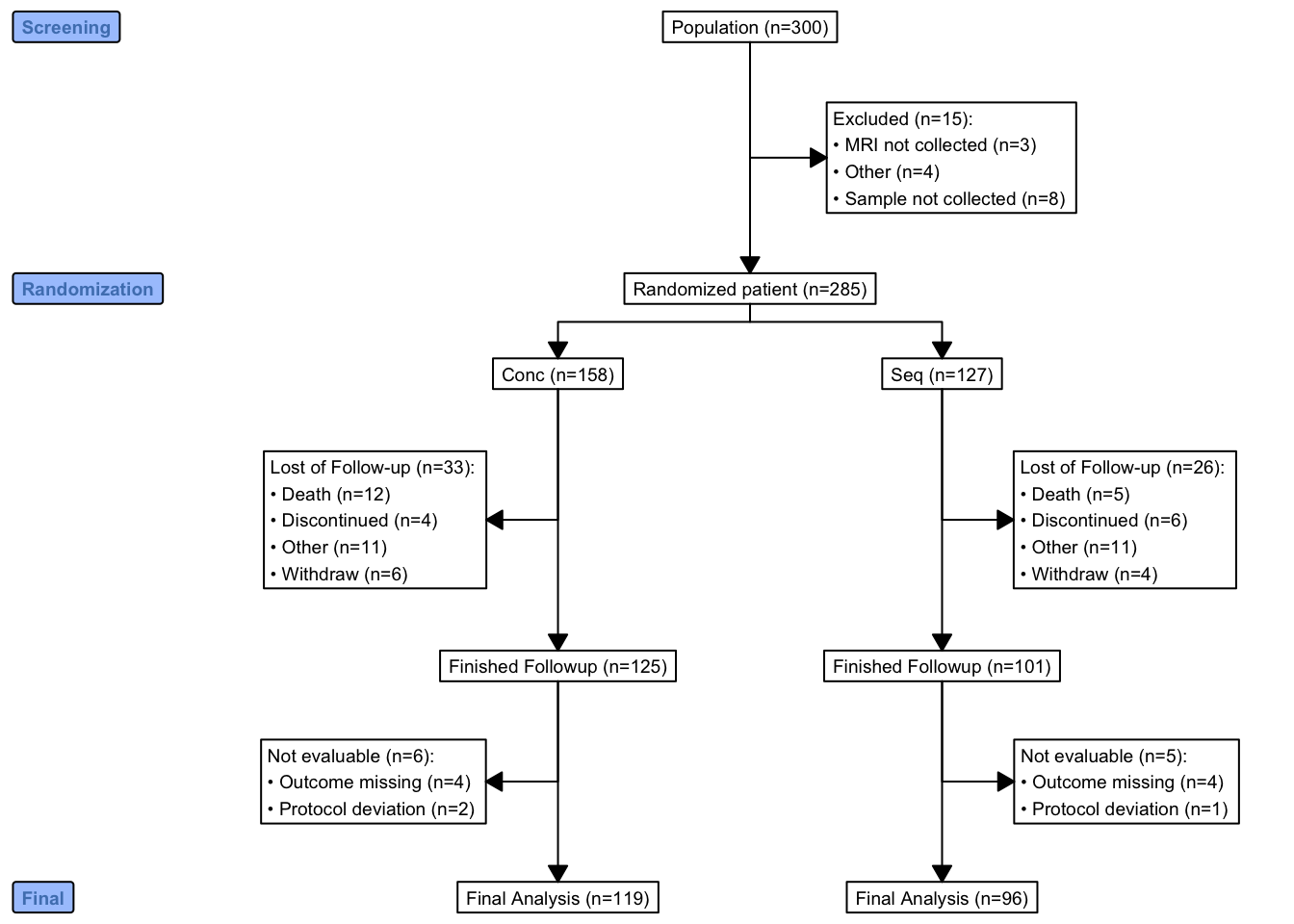

plot(out, grViz = TRUE)

require(Hmisc)
require(data.table)
require(qreport)
hookaddcap()
N <- 1000
set.seed(1)
r <- data.table(
  id    = 1 : N,
  age   = round(rnorm(N, 60, 15)),
  pain  = sample(0 : 5, N, replace=TRUE),
  hxmed = sample(0 : 1, N, replace=TRUE, prob=c(0.95, 0.05))   )
# Set consent status to those not excluded at screening
r[age >= 40 & pain > 0 & hxmed == 0,
  consent := sample(0 : 1, .N, replace=TRUE, prob=c(0.1, 0.9))]
# Set randomization status for those consenting
r[consent == 1,
  randomized := sample(0 : 1, .N, replace=TRUE, prob=c(0.15, 0.85))]
# Add treatment and follow-up time to randomized subjects
r[randomized == 1, tx     := sample(c('A', 'B'), .N, replace=TRUE)]
r[randomized == 1, futime := pmin(runif(.N, 0, 10), 3)]
# Add outcome status for those followed 3 years
# Make a few of those followed 3 years missing
r[futime == 3,
  y := sample(c(0, 1, NA), .N, replace=TRUE, prob=c(0.75, 0.2, 0.05))]
# Print first 15 subjects
kabl(r[1 : 15, ])

id	age	pain	hxmed	consent	randomized	tx	futime	y
1	51	2	1	NA	NA	NA	NA	NA
2	63	2	0	1	1	A	3.0000	0
3	47	1	0	1	1	A	3.0000	NA
4	84	5	0	1	0	NA	NA	NA
5	65	3	0	1	1	B	3.0000	1
6	48	4	0	1	1	A	3.0000	0
7	67	3	0	1	1	B	2.0566	NA
8	71	0	0	NA	NA	NA	NA	NA
9	69	5	0	1	1	B	1.2815	NA
10	55	2	0	1	1	B	1.2388	NA
11	83	4	0	1	1	A	3.0000	1
12	66	5	0	1	1	A	3.0000	0
13	51	1	0	1	1	B	3.0000	0
14	27	2	0	NA	NA	NA	NA	NA
15	77	2	0	1	1	A	3.0000	0

r[, exc := seqFreq('pain-free'  = pain  == 0,
                    'Hx med'    = hxmed == 1,
                                  age < 40,
                    noneNA=TRUE)]
eo  <- attr(r[, exc], 'obs.per.numcond')
mult <- paste0('1, 2, ≥3 exclusions: n=',
                eo[2], ', ',
                eo[3], ', ',
                eo[-(1:3)]  )

r[, .q(qual, consent, fin) :=
    .(is.na(exc),
      ifelse(consent == 1, 1, NA),
      ifelse(futime  >= 3, 1, NA))]
            
require(consort)
# consort_plot used to take a coords=c(0.4, 0.6) argument that prevented
# the collision you see here
consort_plot(r,
             orders = c(id      = 'Screened',
                        exc     = 'Excluded',
                        qual    = 'Qualified for Randomization',
                        consent = 'Consented',
                        tx      = 'Randomized',
                        fin     = 'Finished',
                        y       = 'Outcome\nassessed'),
             side_box = 'exc',
             allocation = 'tx',
             labels=c('1'='Screening', '3'='Consent', '4'='Randomization', '6'='Follow-up'))

htab

h <- function(n, label) paste0(label, ' (n=', n, ')')
htab <- function(x, label=NULL, split=! length(label), br='\n') {
  tab <- table(x)
  w <- if(length(label)) paste0(h(sum(tab), label), ':', br)
  f <- if(split) h(tab, names(tab)) 
  else
    paste(paste0('   ', h(tab, names(tab))), collapse=br)
  if(split) return(f)
  paste(w, f, sep=if(length(label))'' else br)
}  
count <- function(x, by=rep(1, length(x)))
  tapply(x, by, sum, na.rm=TRUE)

w <- r[, {
 g <-
   add_box(txt=h(nrow(r),       'Screened'))                    |>
   add_side_box(htab(exc,       'Excluded'))                    |>
   add_box(h(count(is.na(exc)), 'Qualified for Randomization')) |>
   add_box(h(count(consent),    'Consented'))                   |>
   add_box(h(count(randomized), 'Randomized'))                  |>
   add_split(htab(tx))                                          |>
   add_box(h(count(fin, tx),    'Finished'))                    |>
   add_box(h(count(! is.na(y), tx), 'Outcome\nassessed'))       |>
   add_label_box(c('1'='Screening',     '3'='Consent',
                   '4'='Randomization', '6'='Follow-up'))
 plot(g)
}
]

mermaid maker

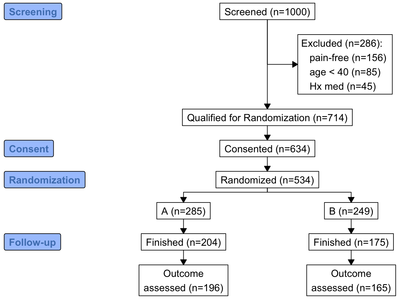
addCap('fig-doverview-mermaid1', 'Consort diagram produced by `mermaid`')
x <- 'flowchart TD
  S["Screened (n={{N0}})"] --> E["{{excl}}"]
  S   --> Q["Qualified for Randomization (n={{Nq}})"]
  Q   --> C["Consented (n={{Nc}})"]
  C   --> R["Randomized (n={{Nr}})"]
  R   --> TxA["A (n={{Ntxa}})"]
  R   --> TxB["B (n={{Ntxb}})"]
  TxA --> FA["Finished (n={{Ntxaf}})"]
  TxB --> FB["Finished (n={{Ntxbf}})"]
  FA  --> OA["Outcome assessed (n={{Ntxao}})"]
  FB  --> OB["Outcome assessed (n={{Ntxbo}})"]
classDef largert fill:lightgray,width:1.5in,height:10em,text-align:right,font-size:0.8em;
class E largert;
'

w <- r[, 
makemermaid(x,
            N0   = nrow(r),
            excl = htab(exc, 'Excluded', br='<br>'),
            Nq   = count(is.na(exc)),
            Nc   = count(consent),
            Nr   = count(randomized),
            Ntxa = count(tx == 'A'),
            Ntxb = count(tx == 'B'),
            Ntxaf= count(tx == 'A' & fin),
            Ntxbf= count(tx == 'B' & fin),
            Ntxao= count(tx == 'A' & ! is.na(y)),
            Ntxbo= count(tx == 'B' & ! is.na(y)),
            file = 'assets/mermaid1.mer'
            )
]

flowchart TD
  S["Screened (n=1000)"] --> E["Excluded (n=286):<br>   pain-free (n=156)<br>   age < 40 (n=85)<br>   Hx med (n=45)"]
  S   --> Q["Qualified for Randomization (n=714)"]
  Q   --> C["Consented (n=634)"]
  C   --> R["Randomized (n=534)"]
  R   --> TxA["A (n=285)"]
  R   --> TxB["B (n=249)"]
  TxA --> FA["Finished (n=204)"]
  TxB --> FB["Finished (n=175)"]
  FA  --> OA["Outcome assessed (n=196)"]
  FB  --> OB["Outcome assessed (n=165)"]
classDef largert fill:lightgray,width:1.5in,height:10em,text-align:right,font-size:0.8em;
class E largert;

Figure 4: Consort diagram produced by mermaid

node plot

# Create some service functions so later it will be easy to change from
# mermaid to graphviz
makenode       <- function(name, label) paste0(name, '["', label, '"]')
makeconnection <- function(from, to)    paste0(from, ' --> ', to)

exclnodes <- function(x, from='E', root='E', seq=FALSE, remain=FALSE) {
  # Create complete node specifications for individual exclusions, each
  # linking to overall exclusion count assumed to be in node root.
  # Set seq=TRUE to make use of the fact that the exclusions were
  # done in frequency priority order so that each exclusion is in
  # addition to the previous one.  Leave seq=FALSE to make all exclusions
  # subservient to root.  Use remain=TRUE to include # obs remaining
    # remain=TRUE assumes noneNA specified to seqFreq
  tab <- table(x)
  i <- 1 : length(tab)
    rem <- if(remain) paste0(', ', length(x) - cumsum(tab), ' remain')
  labels <- paste0(names(tab), ' (n=', tab, rem, ')')
  nodes  <- if(seq) makenode(ifelse(i == 1, paste0(root, '1'), paste0(root, i)),
                             labels)
            else    makenode(paste0(root, i), labels)
  connects <- if(seq) makeconnection(ifelse(i == 1, from, paste0(root, i - 1)),
                                     paste0(root, i))
              else makeconnection(from, paste0(root, i))
   paste(c(nodes, connects), collapse='\n')
}

# Create parallel treatment nodes
# Treatments are assumed to be in order by the tx variable
# and will appear left to right in the diagram
# Treatment node names correspond to that and are Tx1, Tx2, ...
# root: root of new nodes, from: single node name to connect from
# fromparallel: root of connected-from node name which is to be
# expanded by adding the integers 1, 2, ... number of treatments.

Txs <- r[, if(is.factor(tx)) levels(tx) else sort(unique(tx))]

parNodes <- function(counts, root, from=NULL, fromparallel=NULL,
                      label=Txs) {
  if(! identical(names(counts), Txs)) stop('Txs not consistent')
  k <- length(Txs)
  ns <- paste0(' (n=', counts, ')')
   nodenames <- paste0(root, 1 : k)
  nodes <- makenode(nodenames, paste0(label, ns))
  connects <- if(length(fromparallel)) makeconnection(paste0(fromparallel, 1 : k), nodenames)
              else                     makeconnection(from,                        nodenames)
  paste(c(nodes, connects), collapse='\n')
    }

# Create tooltip text from tabulation created by seqFreq earlier
efreq <- data.frame('# Exclusions'= (1 : length(eo)) - 1,
                    '# Subjects'  = eo, check.names=FALSE)
efreq <- subset(efreq, `# Subjects` > 0)
# Convert to text which will be wrapped by the html
excltab <- paste(capture.output(print(efreq, row.names=FALSE)),
                 collapse='\n')


addCap('fig-doverview-mermaid2', 'Consort diagram produced with `mermaid` with individual exclusions linked to the overall exclusions node, and with a tooltip to show more detail')

x <- '
flowchart TD
  S["Screened (n={{N0}})"] --> E["Excluded (n={{Ne}})"]
  {{exclsep}}
  E1 & E2 & E3 --> M["{{mult}}"]
  S   --> Q["Qualified for Randomization (n={{Nq}})"]
  Q   --> C["Consented (n={{Nc}})"]
  C   --> R["Randomized (n={{Nr}})"]
  {{txcounts}}
  {{finished}}
  {{outcome}}
click E callback "{{excltab}}"
'

w <- r[, 
makemermaid(x,
  N0       = nrow(r),
  Ne       = count(! is.na(exc)),
  exclsep  = exclnodes(exc),  # add seq=TRUE to put exclusions vertical
  excltab  = excltab,         # tooltip text
  mult     = mult,  # separate node: count multiple exclusions
  Nq       = count(is.na(exc)),
  Nc       = count(consent),
  Nr       = count(randomized),
  txcounts = parNodes(table(tx),         'Tx', from='R'),
  finished = parNodes(count(fin, by=tx), 'F',  fromparallel='Tx',
                      label='Finished'),
  outcome  = parNodes(count(! is.na(y), by=tx), 'O',
                      fromparallel='F', label='Outcome assessed'),
  file='mermaid2.mer'  # save generated code for another use
)
]


makenode       <- function(name, label) paste0(name, ' [label="', label, '"];')
makeconnection <- function(from, to)    paste0(from, ' -> ', to, ';')

# Create data frame from tabulation created by seqFreq earlier
efreq <- data.frame('# Exclusions'= (1 : length(eo)) - 1,
                    '# Subjects'  = eo, check.names=FALSE)
efreq <- subset(efreq, `# Subjects` > 0)

x <- 'digraph {
  graph [pad="0.5", nodesep="0.5", ranksep="2", splines=ortho]
  //  splines=ortho for square connections
  node  [shape=box, fontsize="30"]
  rankdir=TD;
  S [label="Screened (n={{N0}})"];
  E [label="Excluded (n={{Ne}})"];
  S -> E;
  {{exclsep}}
  M [label="{{mult}}"];
  E1 -> M;
  E2 -> M;
  E3 -> M;
  Q [label="Qualified for Randomization (n={{Nq}})"];
  C [label="Consented (n={{Nc}})"];
  R [label="Randomized (n={{Nr}})"];
  S -> Q;
  Q -> C;
  C -> R;
  {{txcounts}}
  {{finished}}
  {{outcome}}
  efreq [label=<{{efreq}}>];
  M -> efreq [dir=none, style=dotted];
}
'

w <- r[, 
makegraphviz(x,
  N0       = nrow(r),
  Ne       = count(! is.na(exc)),
  exclsep  = exclnodes(exc),  # add seq=TRUE to put exclusions vertical
  efreq    = efreq,
  mult     = mult,  # separate node: count multiple exclusions
  Nq       = count(is.na(exc)),
  Nc       = count(consent),
  Nr       = count(randomized),
  txcounts = parNodes(table(tx),         'Tx', from='R'),
  finished = parNodes(count(fin, by=tx), 'F',  fromparallel='Tx',
                      label='Finished'),
  outcome  = parNodes(count(! is.na(y), by=tx), 'O',
                      fromparallel='F', label='Outcome assessed'),
  file='graphviz.dot'
)
]
#  addCap('fig-doverview-graphviza', 'Consort diagram produced with `graphviz` with detailed exclusion frequencies in a separate node', scap='Consort diagram produced with `graphviz`')

flowchart TD
  S["Screened (n=1000)"] --> E["Excluded (n=286)"]
  E1["pain-free (n=156)"]
E2["age < 40 (n=85)"]
E3["Hx med (n=45)"]
E --> E1
E --> E2
E --> E3
  E1 & E2 & E3 --> M["1, 2, ≥3 exclusions: n=260, 25, 1"]
  S   --> Q["Qualified for Randomization (n=714)"]
  Q   --> C["Consented (n=634)"]
  C   --> R["Randomized (n=534)"]
  Tx1["A (n=285)"]
Tx2["B (n=249)"]
R --> Tx1
R --> Tx2
  F1["Finished (n=204)"]
F2["Finished (n=175)"]
Tx1 --> F1
Tx2 --> F2
  O1["Outcome assessed (n=196)"]
O2["Outcome assessed (n=165)"]
F1 --> O1
F2 --> O2
click E callback " # Exclusions # Subjects
            0        714
            1        260
            2         25
            3          1"

Figure 5: Consort diagram produced with mermaid with individual exclusions linked to the overall exclusions node, and with a tooltip to show more detail

getHdata(support)
setDT(support)
# addCap('fig-doverview-missflow', 'Flowchart of sequential exclusion of observations due to missing values')
vars <-  .q(age, sex, dzgroup, edu, income, meanbp, wblc,
            alb, bili, crea, glucose, bun, urine)
ex <- missChk(support, use=vars, type='seq') # seq: don't make report

# Create tooltip text from tabulation created by seqFreq
oc   <- attr(ex, 'obs.per.numcond')
freq <- data.frame('# Exclusions'= (1 : length(oc)) - 1,
                   '# Subjects'  = oc, check.names=FALSE)
freq <- subset(freq, `# Subjects` > 0)

x <- '
digraph {
  graph [pad="0.5", nodesep="0.5", ranksep="2", splines=ortho]
  //  splines=ortho for square connections
  node  [shape=box, fontsize="30"]
  rankdir=TD;
  Enr [label="Enrolled (n={{N0}})"];
  Enr;
  {{exclsep}}
    Extab [label=<{{excltab}}>];
  Enr:e -> Extab [dir=none];
}
'
makegraphviz(x,
  N0        = nrow(support),
  exclsep   = exclnodes(ex, from='Enr', seq=TRUE, remain=TRUE),
  excltab   = freq,
  file      = 'support.dot'
)

grViz('
graph G {
fontname="Helvetica,Arial,sans-serif"
node [fontname="Helvetica,Arial,sans-serif"]
edge [fontname="Helvetica,Arial,sans-serif"]
I5 [shape=ellipse,color=red,style=bold,label="Caroline Bouvier Kennedy\nb. 27.11.1957 New York",image="images/165px-Caroline_Kennedy.jpg",labelloc=b];
I1 [shape=box,color=blue,style=bold,label="John Fitzgerald Kennedy\nb. 29.5.1917 Brookline\nd. 22.11.1963 Dallas",image="images/kennedyface.jpg",labelloc=b];
I6 [shape=box,color=blue,style=bold,label="John Fitzgerald Kennedy\nb. 25.11.1960 Washington\nd. 16.7.1999 over the Atlantic Ocean, near Aquinnah, MA, USA",image="images/180px-JFKJr2.jpg",labelloc=b];
I7 [shape=box,color=blue,style=bold,label="Patrick Bouvier Kennedy\nb. 7.8.1963\nd. 9.8.1963"];
I2 [shape=ellipse,color=red,style=bold,label="Jaqueline Lee Bouvier\nb. 28.7.1929 Southampton\nd. 19.5.1994 New York City",image="images/jacqueline-kennedy-onassis.jpg",labelloc=b];
I8 [shape=box,color=blue,style=bold,label="Joseph Patrick Kennedy\nb. 6.9.1888 East Boston\nd. 16.11.1969 Hyannis Port",image="images/1025901671.jpg",labelloc=b];
I10 [shape=box,color=blue,style=bold,label="Joseph Patrick Kennedy Jr\nb. 1915\nd. 1944"];
I11 [shape=ellipse,color=red,style=bold,label="Rosemary Kennedy\nb. 13.9.1918\nd. 7.1.2005",image="images/rosemary.jpg",labelloc=b];
I12 [shape=ellipse,color=red,style=bold,label="Kathleen Kennedy\nb. 1920\nd. 1948"];
I13 [shape=ellipse,color=red,style=bold,label="Eunice Mary Kennedy\nb. 10.7.1921 Brookline"];
I9 [shape=ellipse,color=red,style=bold,label="Rose Elizabeth Fitzgerald\nb. 22.7.1890 Boston\nd. 22.1.1995 Hyannis Port",image="images/Rose_kennedy.JPG",labelloc=b];
I15 [shape=box,color=blue,style=bold,label="Aristotle Onassis"];
I3 [shape=box,color=blue,style=bold,label="John Vernou Bouvier III\nb. 1891\nd. 1957",image="images/BE037819.jpg",labelloc=b];
I4 [shape=ellipse,color=red,style=bold,label="Janet Norton Lee\nb. 2.10.1877\nd. 3.1.1968",image="images/n48862003257_1275276_1366.jpg",labelloc=b];
 I1 -- I5  [style=bold,color=blue]; 
 I1 -- I6  [style=bold,color=orange]; 
 I2 -- I6  [style=bold,color=orange]; 
 I1 -- I7  [style=bold,color=orange]; 
 I2 -- I7  [style=bold,color=orange]; 
 I1 -- I2  [style=bold,color=violet]; 
 I8 -- I1  [style=bold,color=blue]; 
 I8 -- I10  [style=bold,color=orange]; 
 I9 -- I10  [style=bold,color=orange]; 
 I8 -- I11  [style=bold,color=orange]; 
 I9 -- I11  [style=bold,color=orange]; 
 I8 -- I12  [style=bold,color=orange]; 
 I9 -- I12  [style=bold,color=orange]; 
 I8 -- I13  [style=bold,color=orange]; 
 I9 -- I13  [style=bold,color=orange]; 
 I8 -- I9  [style=bold,color=violet]; 
 I9 -- I1  [style=bold,color=red]; 
 I2 -- I5  [style=bold,color=red]; 
 I2 -- I15  [style=bold,color=violet]; 
 I3 -- I2  [style=bold,color=blue]; 
 I3 -- I4  [style=bold,color=violet]; 
 I4 -- I2  [style=bold,color=red]; 
}')