The Role of Variability in Learning Generalization: A Computational Modeling Approach
Submitted to the faculty of the Graduate School
in partial fulfillment of the requirements
for the degree
Doctor of Philosophy
in the Cognitive Science Program and
Department of Psychological and Brain Sciences,
Indiana University
October 2024
Accepted by the Graduate Faculty, Indiana University, in partial fulfillment of the requirements for the degree of Doctor of Philosophy.
Doctoral Committee:
_________________________
Robert L. Goldstone, Ph.D.
Robert L. Goldstone, Ph.D.
_________________________
Robert M. Nosofsky, Ph.D.
Robert M. Nosofsky, Ph.D.
_________________________
Peter M. Todd, Ph.D.
Peter M. Todd, Ph.D.
_________________________
Michael N. Jones, Ph.D.
Michael N. Jones, Ph.D.
May 28th, 2024
Copyright © 2024
Thomas E. Gorman
Thomas E. Gorman
Acknowledgements
My dissertation would not have been possible without the support and guidance of numerous individuals who have shaped my academic and personal growth.
First, I owe immense appreciation to my advisor, Rob Goldstone, for his clear thinking and unwavering support, patiently guiding me throughout my dissertation journey. His demonstration of how a single scientist can contribute meaningful work across several distinct areas has been nothing short of inspiring. I also extend my heartfelt thanks to Rob Nosofsky, who always asked sharp questions that challenged my thinking, and to Peter Todd, whose encouragement and enthusiasm played an especially important role during the final stages of my work.
My journey into the study of the mind began at the Learning and Transfer Lab at the University of Wisconsin-Madison, where I am forever indebted to Dr. Shawn Green. He gave me my first research job despite my total lack of experience, and through his guidance, I discovered my passion for research. It was my time in his lab that made it clear to me that pursuing a career in psychological research was what I wanted to do. I also want to thank Aaron Cochrane for investing significant time in answering my many research questions, introducing me to R, and patiently humoring my naïve inquiries into statistics.
The camaraderie, friendship, and intellectual stimulation I received from my friends at Indiana University have been vital to my graduate school experience. I am especially grateful to Johnathan Avery for introducing me to bouldering, which became my main source of exercise, and for our many fun and thought-provoking conversations. I also want to thank Eleanor Schille-Hudson, Mahi Luthra, Dan Levitas, Sam Nordli, Brad Rogers, Marina Dubova, Eeshan Hasan, and many others from the Geolab, Cognitive Science program, and Psychology department for their support, which made the long hours of work much more enjoyable.
I owe much to my teachers at Pardeeville High School for laying the foundation of my education and to the professors at UW-Madison and Indiana University, who continued to foster and build upon that foundation. Their dedication helped to instill in me a love of learning and a drive to pursue knowledge that has lasted throughout my academic journey.
Finally, I would also like to extend my heartfelt thanks to my family. My parents, Mary and Jim Gorman, have been unwavering pillars of support. My brother, Joseph Gorman, played a crucial role in the final stages of my dissertation. By hosting me for one of the final months of my work, he provided a novel and structured working environment that helped me overcome some of the most challenging hurdles. The support of my family has been instrumental in making this journey possible, and I am forever grateful for their love and encouragement.
Abstract
The impact of training variability on generalization has been a long-standing topic in the study of human learning, with conflicting evidence about its potential benefits. This dissertation addresses these ambiguities by examining the effects of varied versus constant training in visuomotor skill learning through a combination of experimental and computational modeling approaches. Across two projects, we systematically compare varied training (multiple items) to constant training (single item) in a projectile-throwing task. Empirical findings reveal both positive and negative impacts of variability, highlighting the complex interplay between training conditions and generalization performance. To provide a theoretical account of these findings, this dissertation employs both instance-based and connectionist computational modeling approaches. The instance-based modeling approach introduced in Project 1 provides a theoretically justifiable method of quantifying and controlling for similarity between training and testing conditions, while also demonstrating that varied training may induce broader generalization in the similarity function relating training and test items. In Project 2, the Extrapolation-Association Model (EXAM) provided the best account of the testing data across all experiments, capturing the constant groups’ ability to extrapolate to novel regions despite limited training experience, while also revealing potential detriments of varied training for simple extrapolation tasks. These results challenge simplistic notions about the universality of variability benefits in training and emphasize the need for tailored approaches that consider both the structure of the task environment and the prior knowledge of the learners.
Table of contents
Introduction
Varied Training and Generalization
Varied training has been shown to influence learning in a wide array of different tasks and domains, including categorization (Hahn et al., 2005; Maddox & Filoteo, 2011; Morgenstern et al., 2019; Nosofsky et al., 2019; Plebanek & James, 2021; Posner & Keele, 1968), language learning (Brekelmans et al., 2022; Jones & Brandt, 2020; Perry et al., 2010; Twomey et al., 2018; Wonnacott et al., 2012), pattern and anagram completion tasks (Goode et al., 2008; Zhang & Fyfe, 2024), perceptual learning (Lovibond et al., 2020; Manenti et al., 2023; Robson et al., 2022; Zaman et al., 2021), trajectory extrapolation (Fulvio et al., 2014), cognitive control tasks (Moshon-Cohen et al., 2024; Sabah et al., 2019), associative learning (Fan et al., 2022; Lee et al., 2019; Livesey & McLaren, 2019; Prada & Garcia-Marques, 2020; Ram et al., 2024; Reichmann et al., 2023), visual search (George & Egner, 2021; Gonzalez & Madhavan, 2011; T. A. Kelley & Yantis, 2009), voice identity learning (Lavan et al., 2019), face recognition (Burton et al., 2016; Honig et al., 2022; Menon et al., 2015), the perception of social group heterogeneity (Gershman & Cikara, 2023; Konovalova & Le Mens, 2020; Linville & Fischer, 1993; Park & Hastie, 1987), simple motor learning (Braun et al., 2009; Roller et al., 2001; Velázquez-Vargas et al., 2024; Willey & Liu, 2018a), sports training (Breslin et al., 2012; Green et al., 1995; North et al., 2019), and complex skill learning (Hacques et al., 2022; Huet et al., 2011; Seow et al., 2019). See Czyż (2021) and Raviv et al. (2022) for more detailed reviews.
Research on the effects of varied training typically manipulates variability in one of two ways. In the first approach, a high variability group is exposed to a greater number of unique instances during training, while a low variability group receives fewer unique instances with more repetitions. Alternatively, both groups may receive the same number of unique instances, but the high variability group’s instances are more widely distributed or spread out in the relevant psychological space, while the low variability group’s instances are clustered more tightly together. Researchers then compare the training groups in terms of their performance during the training phase, as well as their generalization performance during a testing phase. Researchers usually compare the performance of the two groups during both the training phase and a subsequent testing phase. The primary theoretical interest is often to assess the influence of training variability on generalization to novel testing items or conditions. However, the test may also include some or all of the items that were used during the training stage, allowing for an assessment of whether the variability manipulation influenced the learning of the trained items themselves, or to easily measure how much performance degrades as a function of how far away testing items are from the training items.
The influence of training variability has received a large amount of attention in the domain of sensorimotor skill learning. Much of this research has been influenced by the work of Schmidt (1975), who proposed a schema-based account of motor learning as an attempt to address the longstanding problem of how novel movements are produced. Schema theory presumes that learners possess general motor programs for a class of movements (e.g., an underhand throw). When called up for use motor programs are parameterized by schema rules which determine how the motor program is parameterized or scaled to the particular demands of the current task. Schema theory predicts that variable training facilitates the formation of more robust schemas, which will result in improved generalization or transfer. Experiments that test this hypothesis are often designed to compare the transfer performance of a constant-trained group against that of a varied-trained group. Both groups train on the same task, but the varied group practices with multiple instances along some task-relevant dimension that remains invariant for the constant group. For example, studies using a projectile throwing task might assign participants to either constant training that practice throwing from a single location, or to a varied group that throws from multiple locations. Following training, both groups are then tested from novel throwing locations (Pacheco & Newell, 2018; Pigott & Shapiro, 1984; Willey & Liu, 2018a; Wulf, 1991).
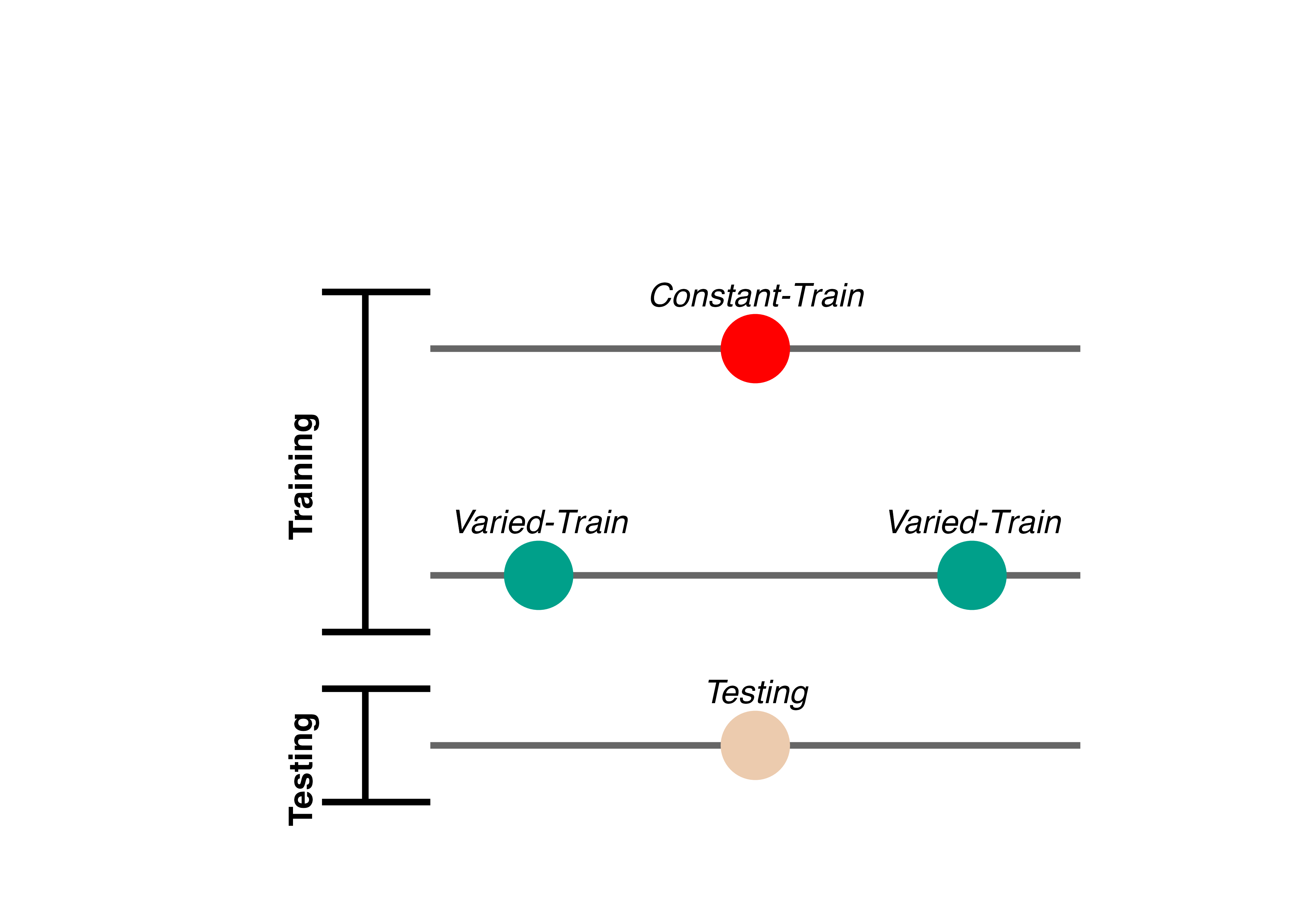
One of the earliest and still often cited investigations of Schmidt’s benefits of variability hypothesis was the work of Kerr & Booth (1978). Two groups of children, aged 8 and 12, were assigned to either constant or varied training of a bean bag throwing task. The constant group practiced throwing a bean-bag at a small target placed 3 feet in front of them, and the varied group practiced throwing from a distance of both 2 feet and 4 feet (see Figure 1). Participants were blindfolded and unable to see the target while making each throw but would receive feedback by looking at where the beanbag had landed in between each training trial. 12 weeks later, all of the children were given a final test from a distance of 3 feet which was novel for the varied participants and repeated for the constant participants. Participants were also blindfolded for testing and did not receive trial by trial feedback in this stage. In both age groups, participants performed significantly better in the varied condition than the constant condition, though the effect was larger for the younger, 8-year-old children. This result provides particularly strong evidence for the benefits of varied practice, as the varied group outperformed the constant group even when tested at the “home-turf” distance that the constant group had exclusively practiced. A similar pattern of results was observed in another study wherein varied participants trained with tennis, squash, badminton, and short-tennis rackets were compared against constant subjects trained with only a tennis racket (Green et al., 1995). One of the testing conditions had subjects repeat the use of the tennis racket, which had been used on all 128 training trials for the constant group, and only 32 training trials for the varied group. Nevertheless, the varied group outperformed the constant group when using the tennis racket at testing, and also performed better in conditions with several novel racket lengths. However, as is the case with many of the patterns commonly observed in the “benefits of variability” literature, the pattern wherein the varied group outperforms the constant group even from the constants group’s home turf has not been consistently replicated. One recent study attempted a near replication of the Kerr & Booth study (Willey & Liu, 2018b), having subjects throw beanbags at a target, with the varied group training from positions (5 and 9 feet) on either side of the constant group (7 feet). This study did not find a varied advantage from the constant training position, though the varied group did perform better at distances novel to both groups. However, this study diverged from the original in that the participants were adults; and the amount of training was much greater (20 sessions with 60 practice trials each, spread out over 5-7 weeks).
Pitting varied against constant practice against each other on the home turf of the constant group provides a compelling argument for the benefits of varied training, as well as an interesting challenge for theoretical accounts that posit generalization to occur as some function of distance. However, despite its appeal this contrast is relatively uncommon in the literature. It is unclear whether this may be cause for concern over publication bias, or just researchers feeling the design is too risky. A far more common design is to have separate constant groups that each train exclusively from each of the conditions that the varied group encounters (Catalano & Kleiner, 1984; Chua et al., 2019; McCracken & Stelmach, 1977; Moxley, 1979; Newell & Shapiro, 1976), or for a single constant group to train from just one of the conditions experienced by the varied participants (Pigott & Shapiro, 1984; Roller et al., 2001; Wrisberg & McLean, 1984; Wrisberg & Mead, 1983). A less common contrast places the constant group training in a region of the task space outside of the range of examples experienced by the varied group, but distinct from the transfer condition (Wrisberg et al., 1987; Wulf & Schmidt, 1997). Of particular relevance to the current work is the early study of Catalano & Kleiner (1984), as theirs was one of the earliest studies to investigate the influence of varied vs. constant training on multiple testing locations of graded distance from the training condition. Participants were trained on coincident timing task, in which subjects observe a series of lightbulbs turning on sequentially at a consistent rate and attempt to time a button response with the onset of the final bulb. The constant groups trained with a single velocity of either 5,7,9, or 11 mph, while the varied group trained from all 4 of these velocities. Participants were then assigned to one of four possible generalization conditions, all of which fell outside of the range of the varied training conditions – 1, 3, 13 or 15 mph. As is often the case, the varied group performed worse during the training phase. In the testing phase, the general pattern was for all participants to perform worse as the testing conditions became further away from the training conditions, but since the drop off in performance as a function of distance was far less steep for the varied group, the authors suggested that varied training induced a decremented generalization gradient, such that the varied participants were less affected by the change between training and testing conditions.
Benefits of varied training have also been observed in many studies outside of the sensorimotor domain. Goode et al. (2008) trained participants to solve anagrams of 40 different words ranging in length from 5 to 11 letters, with an anagram of each word repeated 3 times throughout training, for a total of 120 training trials. Although subjects in all conditions were exposed to the same 40 unique words (i.e. the solution to an anagram), participants in the varied group saw 3 different arrangements for each solution-word, such as DOLOF, FOLOD, and OOFLD for the solution word FLOOD, whereas constant subjects would train on three repetitions of LDOOF (spread evenly across training). Two different constant groups were used. Both constant groups trained with three repetitions of the same word scramble, but for constant group A, the testing phase consisted of the identical letter arrangement to that seen during training (e.g., LDOOF), whereas for constant group B, the testing phase consisted of an arrangement they had not seen during training, thus presenting them with a testing situation similar situation to the varied group. At the testing stage, the varied group outperformed both constant groups, a particularly impressive result, given that constant group A had three prior exposures to the word arrangement (i.e. the particular permutation of letters) which the varied group had not explicitly seen. However varied subjects in this study did not exhibit the typical decrement in the training phase typical of other varied manipulations in the literature, and achieved higher levels of anagram solving accuracy by the end of training than either of the constant groups – solving two more anagrams on average than the constant group. This might suggest that for tasks of this nature where the learner can simply get stuck with a particular word scramble, repeated exposure to the identical scramble might be less helpful towards finding the solution than being given a different arrangement of the same letters. This contention is supported by the fact that constant group A, who was tested on the identical arrangement as they experienced during training, performed no better at testing than did constant group B, who had trained on a different arrangement of the same word solution – further suggesting that there may not have been a strong identity advantage in this task.
In the domain of category learning, the constant vs. varied comparison is much less suitable. Instead, researchers will typically employ designs where all training groups encounter numerous stimuli, but one group experiences a greater number of unique exemplars (Brunstein & Gonzalez, 2011; Doyle & Hourihan, 2016; Hosch et al., 2023; Nosofsky et al., 2019; Wahlheim et al., 2012), or designs where the number of unique training exemplars is held constant, but one group trains with items that are more dispersed, or spread out across the category space (Bowman & Zeithamova, 2020; Homa & Vosburgh, 1976; Hu & Nosofsky, 2024; Maddox & Filoteo, 2011; Posner & Keele, 1968).
Much of the earlier work in this sub-area trained subjects on artificial categories, such as dot patterns (Homa & Vosburgh, 1976; Posner & Keele, 1968). A seminal study by Posner & Keele (1968) trained participants to categorize artificial dot patterns, manipulating whether learners were trained with low variability examples clustered close to the category prototypes (i.e. low distortion training patterns), or higher-variability patterns spread further away from the prototype (i.e. high-distortion patterns). Participants that received training on more highly-distorted items showed superior generalization to novel high distortion patterns in the subsequent testing phase. It should be noted that unlike the sensorimotor studies discussed earlier, the Posner & Keele (1968) study did not present low-varied and high-varied participants with an equal number of training trials, but instead had participants remain in the training stage of the experiment until they reached a criterion level of performance. This train-until-criterion procedure led to the high-variability condition participants tending to complete a larger number of training trials before switching to the testing stage. More recent work (Hu & Nosofsky, 2024) also used dot pattern categories, but matched the number of training trials across conditions. Under this procedure, higher-variability participants tended to reach lower levels of performance by the end of the training stage. The results in the testing phase were the opposite of Posner & Keele (1968), with the low-variability training group showing superior generalization to novel high-distortion patterns (as well as generalization to novel patterns of low or medium distortion levels). However, whether this discrepancy is solely a result of the different training procedures is unclear, as the studies also differed in the nature of the prototype patterns used. Posner & Keele (1968) utilized simpler, recognizable prototypes (e.g., a triangle, the letter M, the letter F), while Hu & Nosofsky (2024) employed random prototype patterns.
Recent studies have also begun utilizing more complex or realistic stimuli when assessing the influence of variability on category learning. Wahlheim et al. (2012) conducted one such study. In a within-participants design, participants were trained on bird categories with either many repetitions of a few exemplars, or with few repetitions of many exemplars. Across four different experiments, which were conducted to address an unrelated question on metacognitive judgements, the researchers consistently found that participants generalized better to novel species following training with more unique exemplars (i.e. higher variability), while high repetition training produced significantly better performance categorizing the specific species they had trained on. A variability advantage was also found in the relatively complex domain of rock categorization (Nosofsky et al., 2019). For 10 different rock categories, participants were trained with either many repetitions of 3 unique examples of each category, or few repetitions of 9 unique examples, with an equal number of total training trials in each group (the design also included 2 other conditions less amenable to considering the impact of variation). The high-variability group, trained with 9 unique examples, showed significantly better generalization performance than the other conditions.
A distinct sub-literature within the category learning domain has examined how the variability or dispersion of the categories themselves influences generalization to ambiguous regions of the category space (e.g., the region between the two categories). The general approach is to train participants with examples from a high variability category and a low variability category. Participants are then tested with novel items located within ambiguous regions of the category space which allow the experimenters to assess whether the difference in category variability influenced how far participants generalize the category boundaries. A. L. Cohen et al. (2001) conducted two experiments with this basic paradigm. In experiment 1, a low variability category composed of 1 instance was compared against a high-variability category of 2 instances in one condition, and 7 instances in another. In experiment 2 both categories were composed of 3 instances, but for the low-variability group the instances were clustered close to each other, whereas the high-variability groups instances were spread much further apart. Participants were tested on an ambiguous novel instance that was located in between the two trained categories. Both experiments provided evidence that participants were much more likely to categorize the novel middle stimulus into the category with greater variation.
Further observations of widened generalization following varied training have since been observed in numerous investigations (Hahn et al., 2005; Hosch et al., 2023; Hsu & Griffiths, 2010; Perlman et al., 2012; Sakamoto et al., 2008; but see Stewart & Chater, 2002; L.-X. Yang & Wu, 2014; and Seitz et al., 2023). The results of Sakamoto et al. (2008) are noteworthy. They first reproduced the basic finding of participants being more likely to categorize an unknown middle stimulus into a training category with higher variability. In a second experiment, they held the variability between the two training categories constant and instead manipulated the training sequence, such that the examples of one category appeared in an ordered fashion, with very small changes from one example to the other (the stimuli were lines that varied only in length), whereas examples in the alternate category were shown in a random order and thus included larger jumps in the stimulus space from trial to trial. They found that the middle stimulus was more likely to be categorized into the category that had been learned with a random sequence, which was attributed to an increased perception of variability which resulted from the larger trial to trial discrepancies.
The work of Hahn et al. (2005), is also of particular interest to the present work. Their experimental design was similar to previous studies, but they included a larger set of testing items which were used to assess generalization both between the two training categories as well as novel items located in the outer edges of the training categories. During generalization testing, participants were given the option to respond with “neither”, in addition to responses to the two training categories. The “neither” response was included to test how far away in the stimulus space participants would continue to categorize novel items as belonging to a trained category. Consistent with prior findings, high-variability training resulted in an increased probability of categorizing items in between the training categories as belong to the high variability category. Additionally, participants trained with higher variability also extended the category boundary further out into the periphery than participants trained with a lower variability category were willing to do. The author compared a variety of similarity-based models based around the Generalized Context Model (Nosofsky, 1986) to account for their results, manipulating whether a response-bias or similarity-scaling parameter was fit separately between variability conditions. No improvement in model fit was found by allowing the response-bias parameter to differ between groups, however the model performance did improve significantly when the similarity scaling parameter was fit separately. The best fitting similarity-scaling parameters were such that the high-variability group was less sensitive to the distances between stimuli, resulting in greater similarity values between their training items and testing items. This model accounted for both the extended generalization gradients of the varied participants, and for their poorer performance in a recognition condition.
Variability has also been examined in the learning of higher-order linguistic categories (Perry et al., 2010). In nine training sessions spread out over nine weeks infants were trained on object labels in a naturalistic play setting. All infants were introduced to three novel objects of the same category, with participants in the “tight” condition being exposed to three similar exemplars of the category, and participants in the varied condition being exposed to three dissimilar objects of the same category. Importantly, the similarity of the objects was carefully controlled for by having a separate group of adult subjects provide pairwise similarity judgements of the category objects prior to the study onset. Multidimensional scaling was then performed to obtain the coordinates of the objects psychological space, and out of the 10 objects for each category, the 3 most similar objects were selected for the tight group and the three least similar objects for the varied group, with the leftover four objects being retained for testing. By the end of the nine weeks, all of the infants had learned the labels of the training objects. In the testing phase, the varied group demonstrated superior ability to correctly generalize the object labels to untrained exemplars of the same category. More interesting was the superior performance of the varied group on a higher order generalization task – such that they were able to appropriately generalize the bias they had learned during training for attending to the shape of objects to novel solid objects, but not to non-solids. The tight training group, on the other hand, tended to overgeneralize the shape bias, leading the researchers to suggest that the varied training induced a more context-sensitive understanding of when to apply their knowledge.
Of course, the relationship between training variability and transfer is unlikely to be a simple function wherein increased variation is always beneficial. Numerous studies have found null, or in some cases negative effects of training variation (DeLosh et al., 1997; Sinkeviciute et al., 2019; Van Rossum, 1990; Wrisberg et al., 1987), and many more have suggested that the benefits of variability may depend on additional factors such as prior task experience, the order of training trials, or the type of transfer being measured (Berniker et al., 2014; Braithwaite & Goldstone, 2015; Hahn et al., 2005; Lavan et al., 2019; North et al., 2019; Sadakata & McQueen, 2014; Zaman et al., 2021).
In an example of a more complex influence of training variation, (Braithwaite & Goldstone, 2015) trained participants on example problems involving the concept of sampling with replacement (SWR). Training consisted of examples that were either highly similar in their semantic context (e.g., all involving people selecting objects) or in which the surface features were varied between examples (e.g., people choosing objects AND objects selected in a sequence). The experimenters also surveyed how much prior knowledge each participant had with SWR. They found that whether variation was beneficial depended on the prior knowledge of the participants – such that participants with some prior knowledge benefited from varied training, whereas participants with minimal prior knowledge performed better after training with similar examples. The authors hypothesized that to benefit from varied examples, participants must be able to detect the structure common to the diverse examples, and that participants with prior knowledge are more likely to be sensitive to such structure, and thus to benefit from varied training. To test this hypothesis more directly, the authors conducted a 2nd experiment, wherein they controlled prior knowledge by exposing some subjects to a short graphical or verbal pre-training lesson, designed to increase sensitivity to the training examples. Consistent with their hypothesis, participants exposed to the structural sensitivity pre-training benefited more from varied training than the controls participants who benefited more from training with similar examples. Interactions between prior experience and the influence of varied training have also been observed in sensorimotor learning (Del Rey et al., 1982; Guadagnoli et al., 1999). Del Rey et al. (1982) recruited participants who self-reported either extensive, or very little experience with athletic activities, and then trained participants on a coincident timing task with either a single constant training velocity, or with one of several varied training procedures. Unsurprisingly, athlete participants had superior performance during training, regardless of condition, and training performance was superior for all subjects in the constant group. Of greater interest is the pattern of testing results from novel transfer conditions. Among the athlete-participants, transfer performance was best for those who received variable training. Non-athletes showed the opposite pattern, with superior performance for those who had constant training.
Existing Theoretical Frameworks
Several theoretical frameworks have been proposed to conceptually explain the effects of varied training on learning and generalization. Schema theory (described in more detail above), posts that varied practice leads to the formation of more flexible motor schemas, which then facilitate generalization (Schmidt, 1975). The desirable difficulties framework (Bjork & Bjork, 2011; Soderstrom & Bjork, 2015) proposes that variable practice conditions may impair initial performance but then enhance longer-term retention and transfer. Similarly, the challenge point framework (Guadagnoli & Lee, 2004) contends that training variation induces optimal learning occurs insofar as it causes the difficulty of practice tasks to be appropriately matched to the learner’s capabilities, but may also be detrimental if the amount of variation causes the task to be too difficult.
While these frameworks offer valuable conceptual accounts, there has been a limited application of computational modeling efforts aimed at quantitatively assessing and comparing the learning and generalization mechanisms which may be underlying the influence of variability in visuomotor skill learning. In contrast, the effects of variability have received more formal computational treatment in other domains, such as category learning Hu & Nosofsky (2024), language learning (Jones & Brandt, 2020), and function learning (DeLosh et al., 1997). A primary goal of the current dissertation is to address this gap by adapting and applying modeling approaches from these other domains to investigate the effects of training variability in visuomotor skill learning and function learning tasks.
The current work
The overarching purpose of this dissertation is to investigate the effects of training variability on learning and generalization within visuomotor skill learning and function learning. Our investigation is structured into two main projects, each employing distinct experimental paradigms and computational modeling frameworks to elucidate how and when variability in training enhances or impedes subsequent generalization.
In Project 1, we investigated the influence of varied practice in a simple visuomotor projectile launching task. Experiments 1 and 2 compared the performance of constant and varied training groups to assess potential benefits of variability on transfer to novel testing conditions. To account for the observed empirical effects, we introduced the Instance-based Generalization with Adaptive Similarity (IGAS) model. IGAS provides a novel computational approach for quantifying the similarity between training experiences and transfer conditions, while also allowing for variability to influence the generalization gradient itself.
Project 2 will focus on the domain of function learning and in particular the issue of extrapolation. Function learning research examines how people acquire and generalize knowledge about continuous input-output relationships, and the factors influencing extrapolation to novel inputs following an initial learning phase. The domain of function learning has yielded influential computational models, including the Associative Learning Model (ALM) and the Extrapolation-Association Model (EXAM)(Busemeyer et al., 1997), which have successfully accounted for human learning, interpolation, and extrapolation in numerous investigations(DeLosh et al., 1997; McDaniel et al., 2009; McDaniel & Busemeyer, 2005). However, the influence of training variability on function learning, particularly in visuomotor function learning tasks, remains relatively unexplored. Project 2 of this dissertation will address this gap by investigating how constant and varied training regimes affect learning, discrimination, and extrapolation in a novel visuomotor function learning task. We will leverage the ALM and EXAM models, fitted to individual participant data using advanced Bayesian techniques, to provide a detailed computational account of the observed empirical patterns.
Project 1
This project is based on the following publication:
Gorman, T. E., & Goldstone, R. L. (2022). An instance-based model account of the benefits of varied practice in visuomotor skill. Cognitive Psychology, 137, 101491.
Abstract
Exposing learners to variability during training has been demonstrated to improve performance in subsequent transfer testing. Such variability benefits are often accounted for by assuming that learners are developing some general task schema or structure. However, much of this research has neglected to account for differences in similarity between varied and constant training conditions. In a between-groups manipulation, we trained participants on a simple projectile launching task, with either varied or constant conditions. We replicate previous findings showing a transfer advantage of varied over constant training. Furthermore, we show that a standard similarity model is insufficient to account for the benefits of variation, but, if the model is adjusted to assume that varied learners are tuned towards a broader generalization gradient, then a similarity-based model is sufficient to explain the observed benefits of variation. Our results therefore suggest that some variability benefits can be accommodated within instance-based models without positing the learning of some schemata or structure.
Introduction
Similarity and instance-based approaches to transfer of learning
Early models of learning often assumed that discrete experiences with some task or category were not stored individually in memory, but instead promoted the formation of a summary representation, often referred to as a prototype or schema, and that exposure to novel examples would then prompt the retrieval of whichever preexisting prototype was most similar. In addition to being a landmark study on the influence of training variability, Posner & Keele (1968) (described above) also put forward an influential argument concerning the nature of the mental representations acquired during learning - namely that learners tend to abstract a prototype, or aggregate representation of the dot pattern categories, rather than encoding each individual stimulus. Recall that participants are trained on only on distortions of the category prototypes (e.g., low, medium or high distortions), never encountering the exact prototypes during the training stage. Then, in the testing phase, participants are tested with the prototype patterns, their old training items, and novel low, medium and high distortions. The authors found that participants had the highest testing accuracy for the previously unseen prototype patterns, followed by the old training items, and then the novel low, medium and high distortions. The authors interpreted this pattern as evidence that participants had acquired prototype representation of the category, as opposed to storing each individual training instance, and that generalization was based on the similarity of the testing items to the learned prototype representations. Posner & Keele (1968) has been extremely influential, and continues to be cited as evidence that prototype abstraction underlies the benefits of varied training. It’s also referenced as a key influence in the development of the “Schema Theory of Motor Learning” Schmidt (1975), which in turn influenced decades of research on the potential benefits of varied training in motor skill learning. However, a number of the core assumptions utilized by Posner & Keele (1968) were later called into question both empirically and with competing theoretical accounts (Hintzman, 1984, 1986; Knapp & Anderson, 1984; McClelland & Rumelhart, 1985; Nosofsky & Kruschke, 1992; Palmeri & Nosofsky, 2001; Zaki & Nosofsky, 2007). Palmeri & Nosofsky (2001) demonstrated both the dangers of assuming that psychological representations mimic the metric stimulus space, as well the viability of models with simpler representational assumptions. These authors conducted a near replication of the Posner & Keele (1968) study, but also had participants provide similarity judgements of the dot pattern stimuli after completing the training phase. A multidimensional scaling analysis of the similarity judgements revealed that the psychological representations of the prototype stimuli were not located in the middle of the training stimuli, but were instead extreme points in the psychological space. The authors also demonstrated the generalization patterns of Posner & Keele (1968) could be accounted for by an exemplar-based model, without any need to assume the abstraction of a prototype.
Instance-based, or exemplar-based models generally assume that learners encode each experience with a task as a separate instance/exemplar/trace, and that each encoded trace is in turn compared against novel stimuli (Estes, 1994; Hintzman, 1984; Jamieson et al., 2022; Medin & Schaffer, 1978; Nosofsky, 1986). As the number of stored instances increases, so does the likelihood that some previously stored instance will be retrieved to aid in the performance of a novel task. Stored instances are retrieved in the context of novel stimuli or tasks if they are sufficiently similar, thus suggesting that the process of computing similarity is of central importance to generalization.
Similarity, defined in this literature as a function of psychological distance between instances or categories, has provided a successful account of generalization across numerous tasks and domains. In an influential study demonstrating an ordinal similarity effect, experimenters employed a numerosity judgment task in which participants quickly report the number of dots flashed on a screen. Performance (in terms of response times to new patterns) on novel dot configurations varied as an inverse function of their similarity to previously trained dot configurations Palmeri (1997). That is, performance was better on novel configurations moderately similar to trained configurations than to configurations with low-similarity, and also better on low-similarity configurations than to even less similar, unrelated configurations. Instance-based similarity approaches have had some success accounting for performance in certain sub-domains of motor learning (R. G. Cohen & Rosenbaum, 2004; Crump & Logan, 2010; Meigh et al., 2018; Poldrack et al., 1999; Wifall et al., 2017). Crump & Logan (2010) trained participants to type words on an unfamiliar keyboard, while constraining the letters composing the training words to a pre-specified letter set. Following training, typing speed was tested on previously experienced words composed of previously experienced letters; novel words composed of letters from the trained letter set; and novel words composed of letters from an untrained letter set. Consistent with an instance-based account, transfer performance was graded such that participants were fastest at typing the words they had previously trained on, followed by novel words composed of letters they had trained on, and slowest performance for new words composed of untrained letters.
Issues with Previous Research
Although the benefits of training variation in visuomotor skill learning have been observed many times, null findings have also been repeatedly found, leading some researchers to question the veracity of the variability of practice hypothesis (Newell, 2003; Van Rossum, 1990). Critics have also pointed out that investigations of the effects of training variability, of the sort described above, often fail to control for the effect of similarity between training and testing conditions. For training tasks in which participants have numerous degrees of freedom (e.g., projectile throwing tasks where participants control the x and y velocity of the projectile), varied groups are likely to experience a wider range of the task space over the course of their training (e.g., more unique combinations of x and y velocities). Experimenters may attempt to account for this possibility by ensuring that the training location(s) of the varied and constant groups are an equal distance away from the eventual transfer locations, such that their training throws are, on average, equally similar to throws that would lead to good performance at the transfer locations. However, even this level of experimental control may still be insufficient to rule out the effect of similarity on transfer. Given that psychological similarity is typically best described as either a Gaussian or exponentially decaying function of psychological distance (Ennis et al., 1988; Ghahramani et al., 1996; Logan, 1988; Nosofsky, 1992; Shepard, 1987; Thoroughman & Taylor, 2005), it is plausible that a subset of the most similar training instances could have a disproportionate impact on generalization to transfer conditions, even if the average distance between training and transfer conditions is identical between groups. Figure 2 demonstrates the consequences of a generalization gradient that drops off as a Gaussian function of distance from training, as compared to a linear drop-off.

In addition to largely overlooking the potential for non-linear generalization to confound interpretations of training manipulations, the visuomotor skill learning literature also rarely considers alternatives to schema representations (Chamberlin & Magill, 1992b). Although schema-theory remains influential within certain literatures, instance or exemplar-based models have accounted for human behavior across myriad domains (Jamieson et al., 2022; Logan, 2002). As mentioned above, instance based accounts have been shown to perform well on a variety of different tasks with motoric components (Crump & Logan, 2010; Gandolfo et al., 1996; Meigh et al., 2018; Rosenbaum et al., 1995; van Dam & Ernst, 2015). However, such accounts have received little attention within the subdomain of visuomotor skill learning focused on the benefits of varied training.
The present work examines whether the commonly observed benefits of varied training can be accounted for by a theoretically motivated measure of the similarity between training throws and the testing solution space. We first attempt to replicate previous work finding an advantage of varied training over constant training in a projectile launching task. We then examine the extent to which this advantage can be explained by an instance-based similarity model.
Experiment 1
Methods
Sample Size Estimation
To obtain an independent estimate of effect size, we identified previous investigations which included between-subjects contrasts of varied and constant conditions following training on an accuracy-based projectile launching task (Chua et al., 2019; Goodwin et al., 1998; Kerr & Booth, 1978; Wulf, 1991). We then averaged effects across these studies, yielding a Cohen’s f =.43. The GPower 3.1 software package (Faul et al., 2009) was then used to determine that a power of 80% requires a sample size of at least 23 participants per condition. All experiments reported in the present manuscript exceed this minimum number of participants per condition.
Participants
Participants were recruited from an undergraduate population that is 63% female and consists almost entirely of individuals aged 18 to 22 years. A total of 110 Indiana University psychology students participated in Experiment 1. We subsequently excluded 34 participants for poor performance on one of the dependent measures of the task (2.5-3 standard deviations worse than the median subject at the task) or for displaying a pattern of responses that was clearly indicative of a lack of engagement with the task (e.g., simply dropping the ball on each trial rather than throwing it at the target), or for reporting that they completed the experiment on a phone or tablet device, despite the instructions not to use one of these devices. A total of 74 participants were retained for the final analyses, 35 in the varied group and 39 in the constant group.
Task
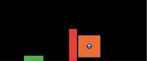
The experimental task was programmed in JavaScript, using packages from the Phaser physics engine (https://phaser.io) and the jsPsych library (de Leeuw, 2015). The stimuli, presented on a black background, consisted of a circular blue ball - controlled by the participant via the mouse or trackpad cursor; a rectangular green target; a red rectangular barrier located between the ball and the target; and an orange square within which the participant could control the ball before releasing it in a throw towards the target. Because the task was administered online, the absolute distance between stimuli could vary depending on the size of the computer monitor being used, but the relative distance between the stimuli was held constant. Likewise, the distance between the center of the target and the training and testing locations was scaled such that relative distances were preserved regardless of screen size. For the sake of brevity, subsequent mentions of this relative distance between stimuli, or the position where the ball landed in relation to the center of the target, will be referred to simply as distance. Figure 3 displays the layout of the task, as it would appear to a participant at the start of a trial, with the ball appearing in the center of the orange square. Using a mouse or trackpad, participants click down on the ball to take control of the ball, connecting the movement of the ball to the movement of the cursor. Participants can then “wind up” the ball by dragging it (within the confines of the orange square) and then launch the ball by releasing the cursor. If the ball does not land on the target, participants are presented with feedback in red text at the top right of the screen, specifying how many scaled units away the ball was from the center of the target. If the ball was thrown outside of the boundary of the screen participants are given feedback as to how far away from the target center the ball would have been if it had continued its trajectory. If the ball strikes the barrier (from the side or by landing on top), feedback is presented telling participants to avoid hitting the barrier. If participants drag the ball outside of the orange square before releasing it, the trial terminates, and they are reminded to release the ball within the orange square. If the ball lands on the target, feedback is presented in green text, confirming that the target was hit, and presenting additional feedback on how many units away the ball was from the exact center of the target.
Link to abbreviated example of task.
Procedure
Participants first electronically consented to participate, and then read instructions for the task which explained how to control the ball, and the goal of throwing the ball as close to the center of the target as possible. The training phase was split into 10 blocks of 20 trials, for a total of 200 training trials. Participants in the constant condition trained exclusively from a single location (760 scaled units from the target center). Participants in the varied condition trained from two locations (610 and 910 scaled units from the target center), encountering each location 100 times. The sequence of throwing locations was pseudo-random for the varied group, with the constraint that within every block of 20 training throws both training locations would occur 10 times. Participants in both conditions also received intermittent testing trials after every 20 training trials. Intermittent testing trials provided no feedback of any kind. The ball would disappear from view as soon as it left the orange square, and participants were prompted to start the next trial without receiving any information about the accuracy of the throw. Each intermittent testing stage consisted of two trials from each of the three training positions (i.e. all participants executed two trials each from Positions 610, 760, and 910 during each of the 10 intermittent testing stages). Following training, all participants completed a final testing phase from four positions: 1) their training location, 2) the training location(s) of the other group, 3) a location novel to both groups. The testing phase consisted of 15 trials from each of the four locations, presented in a randomized order. All trials in the final testing phase included feedback. After finishing the final testing portion of the study, participants were queried as to whether they completed the study using a mouse, a trackpad, or some other device (this information was used in the exclusion process described above). Finally, participants were debriefed as to the hypotheses and manipulation of the study.
Results
Data Processing and Statistical Packages
To prepare the data, we removed trials that were not easily interpretable as performance indicators in our task. Removed trials included: 1) those in which participants dragged the ball outside of the orange starting box without releasing it, 2) trials in which participants clicked on the ball, and then immediately released it, causing the ball to drop straight down, 3) outlier trials in which the ball was thrown more than 2.5 standard deviations further than the average throw (calculated separately for each throwing position), and 4) trials in which the ball struck the barrier. The primary measure of performance used in all analyses was the absolute distance away from the center of the target. The absolute distance was calculated on every trial, and then averaged within each subject to yield a single performance score, for each position. A consistent pattern across training and testing phases in both experiments was for participants to perform worse from throwing positions further away from the target – a pattern which we refer to as the difficulty of the positions. However, there were no interactions between throwing position and training conditions, allowing us to collapse across positions in cases where contrasts for specific positions were not of interest. All data processing and statistical analyses were performed in R version 4.32 (Team, 2020). ANOVAs for group comparisons were performed using the rstatix package (Kassambara, 2021).
Training Phase
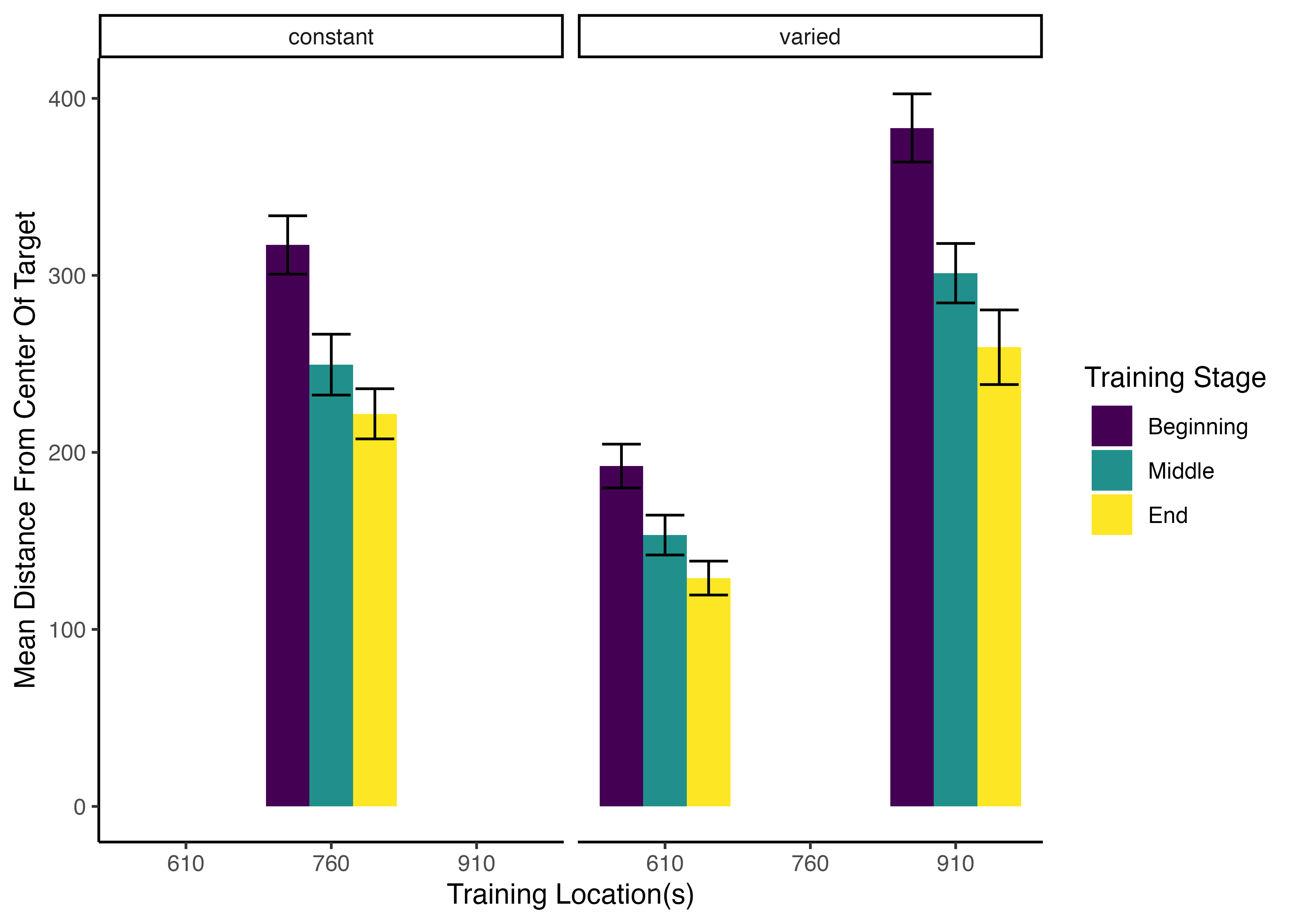
Figure 4 below shows aggregate training performance binned into three stages representing the beginning, middle, and end of the training phase. Because the two conditions trained from target distances that were not equally difficult, it was not possible to directly compare performance between conditions in the training phase. Our focus for the training data analysis was instead to establish that participants did improve their performance over the course of training, and to examine whether there was any interaction between training stage and condition. Descriptive statistics for the intermittent testing phase are provided in the supplementary materials.
We performed an ANOVA comparison with stage as a within-group factor and condition as between-group factor. The analysis revealed a significant effect of training stage F(2,142)=62.4, p<.001, \(\eta^{2}_G\) = .17, such that performance improved over the course of training. There was no significant effect of condition F(1,71)=1.42, p=.24, \(\eta^{2}_G\) = .02, and no significant interaction between condition and training stage, F(2,142)=.10, p=.91, \(\eta^{2}_G\) < .01.
Testing Phase
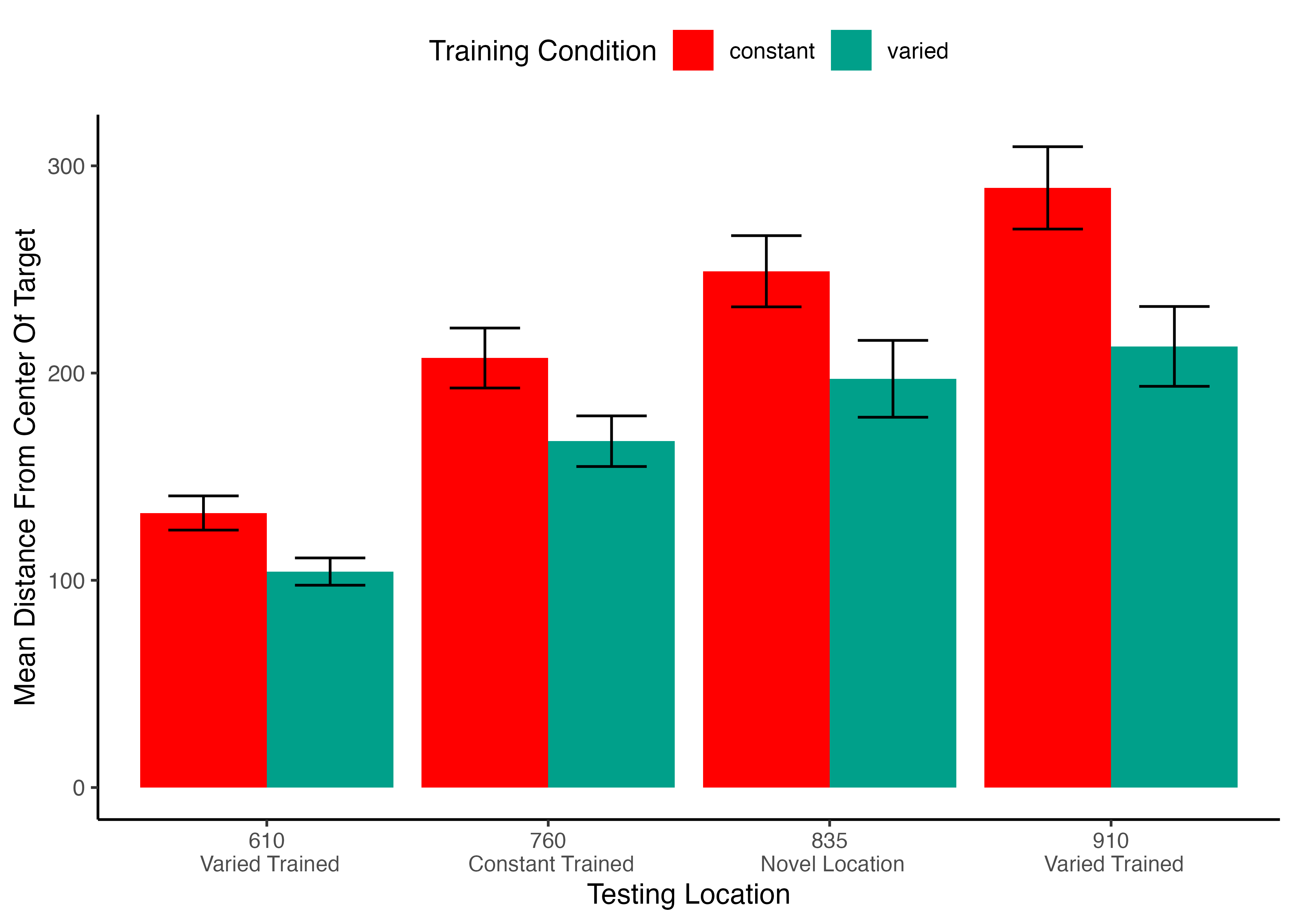
In Experiment 1, a single constant-trained group was compared against a single varied-trained group. At the transfer phase, all participants were tested from 3 positions: 1) the positions(s) from their own training, 2) the training position(s) of the other group, and 3) a position novel to both groups. Overall, group performance was compared with a mixed type III ANOVA, with condition (varied vs. constant) as a between-subject factor and throwing location as a within-subject variable. The effect of throwing position was strong, F(3,213) = 56.12, p<.001, η2G = .23. The effect of training condition was significant F(1,71)=8.19, p<.01, η2G = .07. There was no significant interaction between group and position, F(3,213)=1.81, p=.15, η2G = .01.
| Position | Constant | Varied |
|---|---|---|
| 610 | 132.48(50.85) | 104.2(38.92) |
| 760 | 207.26(89.19) | 167.12(72.29) |
| 835 | 249.13(105.92) | 197.22(109.71) |
| 910 | 289.36(122.48) | 212.86(113.93) |
Discussion
In Experiment 1, we found that varied training resulted in superior testing performance than constant training, from both a position novel to both groups, and from the position at which the constant group was trained, which was novel to the varied condition. The superiority of varied training over constant training even at the constant training position is of particular note, given that testing at this position should have been highly similar for participants in the constant condition. It should also be noted, though, that testing at the constant trained position is not identical to training from that position, given that the context of testing is different in several ways from that of training, such as the testing trials from the different positions being intermixed, as well as a simple change in context as a function of time. Such contextual differences will be further considered in the General Discussion.
In addition to the variation of throwing position during training, the participants in the varied condition of Experiment 1 also received training practice from the closest/easiest position, as well as from the furthest/most difficult position that would later be encountered by all participants during testing. The varied condition also had the potential advantage of interpolating both of the novel positions from which they would later be tested. Experiment 2 thus sought to address these issues by comparing a varied condition to multiple constant conditions.
Experiment 2
In Experiment 2, we sought to replicate our findings from Experiment 1 with a new sample of participants, while also addressing the possibility of the pattern of results in Experiment 1 being explained by some idiosyncrasy of the particular training location of the constant group relative to the varied group. To this end, Experiment 2 employed the same basic procedure as Experiment 1, but was designed with six separate constant groups each trained from one of six different locations (400, 500, 625, 675, 800, or 900), and a varied group trained from two locations (500 and 800). Participants in all seven groups were then tested from each of the 6 unique positions.
Methods
Participants
A total of 306 Indiana University psychology students participated in Experiment 2, which was also conducted online. As was the case in Experiment 1, the undergraduate population from which we recruited participants was 63% female and primarily composed of 18–22-year-old individuals. Using the same procedure as Experiment 1, we excluded 98 participants for exceptionally poor performance at one of the dependent measures of the task, or for displaying a pattern of responses indicative of a lack of engagement with the task. A total of 208 participants were included in the final analyses with 31 in the varied group and 32, 28, 37, 25, 29, 26 participants in the constant groups training from location 400, 500, 625, 675, 800, and 900, respectively. All participants were compensated with course credit.
Task and Procedure
The task of Experiment 2 was identical to that of Experiment 1, in all but some minor adjustments to the height of the barrier, and the relative distance between the barrier and the target. Additionally, the intermittent testing trials featured in experiment 1 were not utilized in Experiment 2. An abbreviated demo of the task used for Experiment 2 can be found at (https://pcl.sitehost.iu.edu/tg/demos/igas_expt2_demo.html).
The procedure for Experiment 2 was also quite similar to Experiment 1. Participants completed 140 training trials, all of which were from the same position for the constant groups and split evenly (70 trials each - randomized) for the varied group. In the testing phase, participants completed 30 trials from each of the six locations that had been used separately across each of the constant groups during training. Each of the constant groups thus experienced one trained location and five novel throwing locations in the testing phase, while the varied group experiences 2 previously trained, and 4 novel locations.
Results
Data Processing and Statistical Packages
After confirming that condition and throwing position did not have any significant interactions, we standardized performance within each position, and then average across position to yield a single performance measure per participant. This standardization did not influence our pattern of results. As in Experiment 1, we performed type III ANOVAs due to our unbalanced design, however the pattern of results presented below is not altered if type 1 or type III tests are used instead. The statistical software for the primary analyses was the same as for Experiment 1. Individual learning rates in the testing phase, compared between groups in the supplementary analyses, were fit using the TEfit package in R (Cochrane, 2020).
Training Phase
The different training conditions trained from positions that were not equivalently difficult and are thus not easily amenable to comparison. As previously stated, the primary interest of the training data is confirmation that some learning did occur. Figure 6 depicts the training performance of the varied group alongside that of the aggregate of the six constant groups (5a), and each of the 6 separate constant groups (5b). An ANOVA comparison with training stage (beginning, middle, end) as a within-group factor and group (the varied condition vs. the 6 constant conditions collapsed together) as a between-subject factor revealed no significant effect of group on training performance, F(1,206)=.55,p=.49, \(\eta^{2}_G\) <.01, a significant effect of training stage F(2,412)=77.91, p<.001, \(\eta^{2}_G\) =.05, and no significant interaction between group and training stage, F(2,412)=.489 p=.61, \(\eta^{2}_G\) <.01. We also tested for a difference in training performance between the varied group and the two constant groups that trained matching throwing positions (i.e., the constant groups training from position 500, and position 800). The results of our ANOVA on this limited dataset mirrors that of the full-group analysis, with no significant effect of group F(1,86)=.48, p=.49, \(\eta^{2}_G\) <.01, a significant effect of training stage F(2,172)=56.29, p<.001, \(\eta^{2}_G\) =.11, and no significant interaction between group and training stage, F(2,172)=.341 p=.71, \(\eta^{2}_G\) <.01.

Testing Phase
In Experiment 2, a single varied condition (trained from two positions, 500 and 800), was compared against six separate constant groups (trained from a single position, 400, 500, 625, 675, 800 or 900). For the testing phase, all participants were tested from all six positions, four of which were novel for the varied condition, and five of which were novel for each of the constant groups. For a general comparison, we took the absolute deviations for each throwing position and computed standardized scores across all participants, and then averaged across throwing position. The six constant groups were then collapsed together allowing us to make a simple comparison between training conditions (constant vs. varied). A type III between-subjects ANOVA was performed, yielding a significant effect of condition F(1,206)=4.33, p=.039, \(\eta^{2}_G\) =.02. Descriptive statistics for each condition are shown in table 2. In Figure 7 visualizes the consistent advantage of the varied condition over the constant groups across the testing positions. Figure 7 shows performance between the varied condition and the individual constant groups.
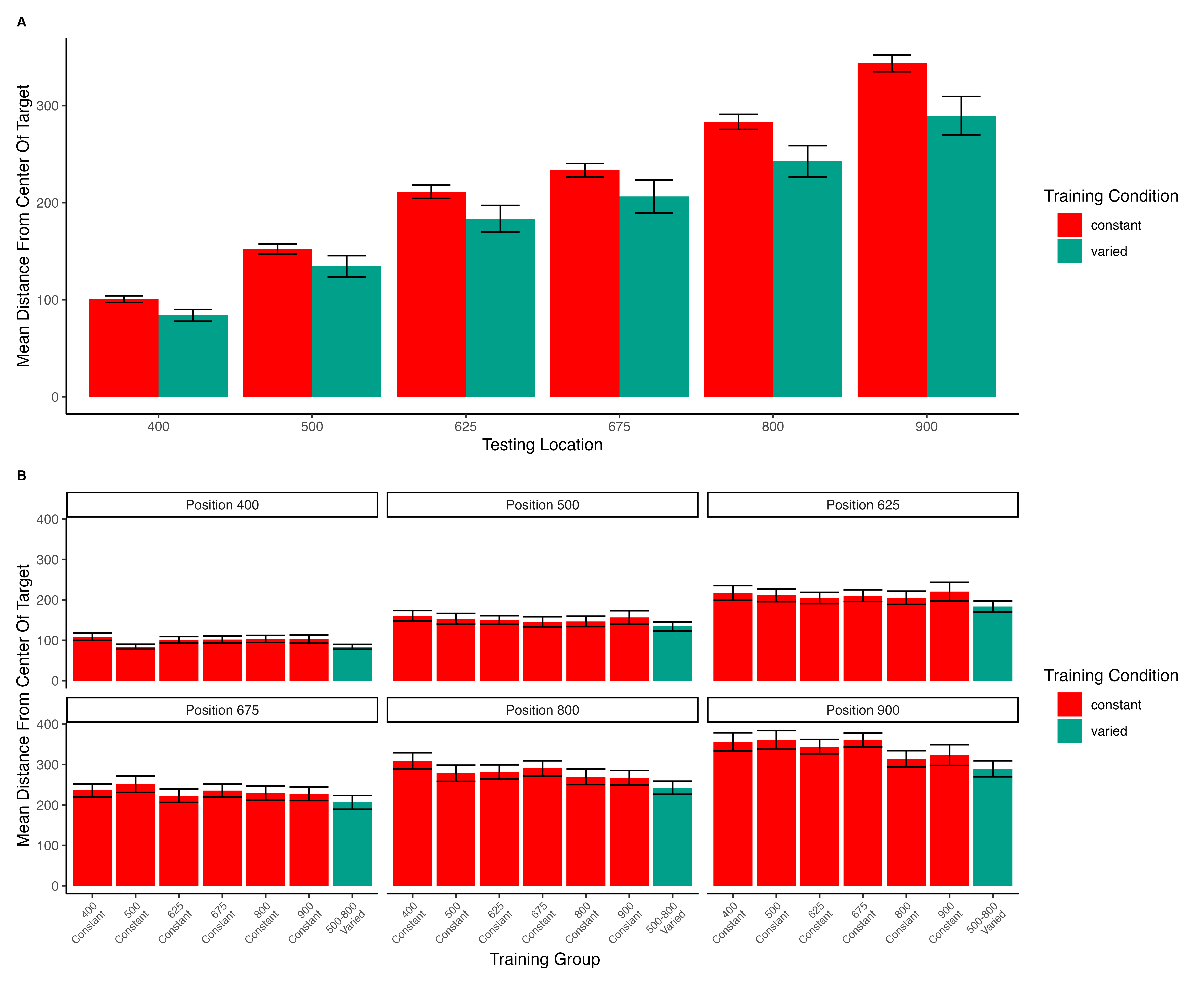
| Position | Constant | Varied |
|---|---|---|
| 400 | 100.59(46.3) | 83.92(33.76) |
| 500 | 152.28(69.82) | 134.38(61.38) |
| 625 | 211.21(90.95) | 183.51(75.92) |
| 675 | 233.32(93.35) | 206.32(94.64) |
| 800 | 283.24(102.85) | 242.65(89.73) |
| 900 | 343.51(114.33) | 289.62(110.07) |
Next, we compared the testing performance of constant and varied groups from only positions that participants had not encountered during training. Constant participants each had 5 novel positions, whereas varied participants tested from 4 novel positions (400,625,675,900). We first standardized performance within in each position, and then averaged across positions. Here again, we found a significant effect of condition (constant vs. varied): F(1,206)=4.30, p=.039, \(\eta^{2}_G\) = .02 .
| Position | Constant | Varied |
|---|---|---|
| 400 | 98.84(45.31) | 83.92(33.76) |
| 500 | 152.12(69.94) | NA |
| 625 | 212.91(92.76) | 183.51(75.92) |
| 675 | 232.9(95.53) | 206.32(94.64) |
| 800 | 285.91(102.81) | NA |
| 900 | 346.96(111.35) | 289.62(110.07) |
Finally, corresponding to the comparison of position 760 from Experiment 1, we compared the test performance of the varied group against the constant group from only the positions that the constant groups trained. Such positions were novel to the varied group (thus this analysis omitted two constant groups that trained from positions 500 or 800 as those positions were not novel to the varied group). Figure 8 displays the subset of comparisons utilized for this analysis. Again, we standardized performance within each position before performing the analyses on the aggregated data. In this case, the effect of condition did not reach statistical significance F(1,149)=3.14, p=.079, \(\eta^{2}_G\) = .02. Table 4 provides descriptive statistics.
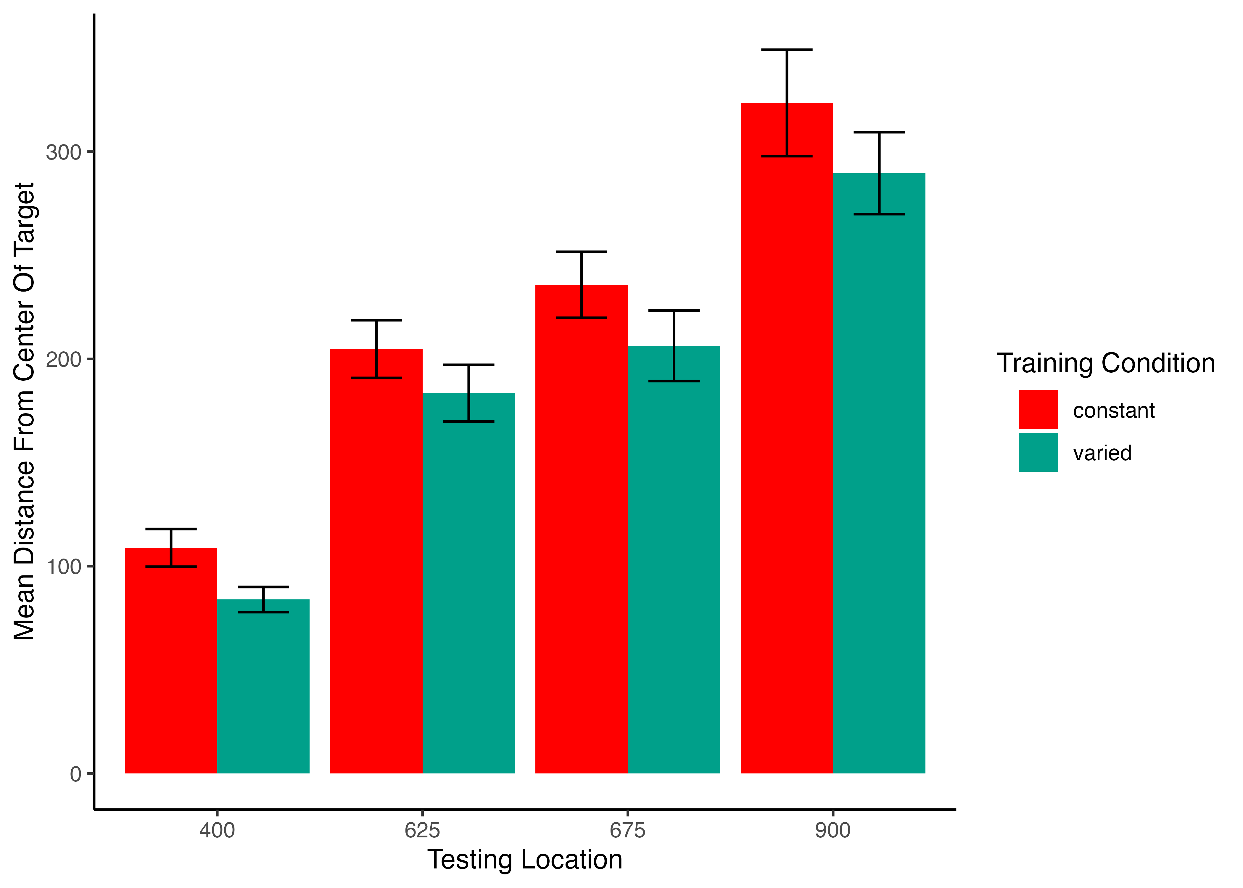
| Position | Constant | Varied |
|---|---|---|
| 400 | 108.85(50.63) | 83.92(33.76) |
| 625 | 204.75(84.66) | 183.51(75.92) |
| 675 | 235.75(81.15) | 206.32(94.64) |
| 900 | 323.5(130.9) | 289.62(110.07) |
Experiment 2 Discussion
The results of Experiment 2 largely conform to the findings of Experiment 1. Participants in both varied and constant conditions improved at the task during the training phase. We did not observe the common finding of training under varied conditions producing worse performance during acquisition than training under constant conditions (Catalano & Kleiner, 1984; Wrisberg et al., 1987), which has been suggested to relate to the subsequent benefits of varied training in retention and generalization testing (Soderstrom & Bjork, 2015). However, our finding of no difference in training performance between constant and varied groups has been observed in previous work (Chua et al., 2019; Moxley, 1979; Pigott & Shapiro, 1984).
In the testing phase, our varied group significantly outperformed the constant conditions in both a general comparison, and in an analysis limited to novel throwing positions. The observed benefit of varied over constant training echoes the findings of many previous visuomotor skill learning studies that have continued to emerge since the introduction of Schmidt’s influential Schema Theory (Catalano & Kleiner, 1984; Chua et al., 2019; Goodwin et al., 1998; McCracken & Stelmach, 1977; Moxley, 1979; Newell & Shapiro, 1976; Pigott & Shapiro, 1984; Roller et al., 2001; Schmidt, 1975; Willey & Liu, 2018b; Wrisberg et al., 1987; Wulf, 1991). We also join a much smaller set of research to observe this pattern in a computerized task (Seow et al., 2019). One departure from the experiment 1 findings concerns the pattern wherein the varied group outperformed the constant group even from the training position of the constant group, which was significant in experiment 1, but did not reach significance in experiment 2. Although this pattern has been observed elsewhere in the literature (Goode et al., 2008; Kerr & Booth, 1978), the overall evidence for this effect appears to be far weaker than for the more general benefit of varied training in conditions novel to all training groups.
Computational Model
Controlling for the similarity between training and testing. The primary goal of Experiment 2 was to examine whether the benefits of variability would persist after accounting for individual differences in the similarity between trained and tested throwing locations. To this end, we modelled each throw as a two-dimensional point in the space of x and y velocities applied to the projectile at the moment of release. For each participant, we took each individual training throw, and computed the similarity between that throw and the entire population of throws within the solution space for each of the 6 testing positions. We defined the solution space empirically as the set of all combinations of x and y throw velocities that resulted in hitting the target. We then summed each of the trial-level similarities to produce a single similarity for each testing position score relating how the participant threw the ball during training and the solutions that would result in target hits from each of the six testing positions – thus resulting in six separate similarity scores for each participant. Figure 9 visualizes the solution space for each location and illustrates how different combinations of x and y velocity result in successfully striking the target from different launching positions. As illustrated in Figure 9, the solution throws represent just a small fraction of the entire space of velocity combinations used by participants throughout the experiment.
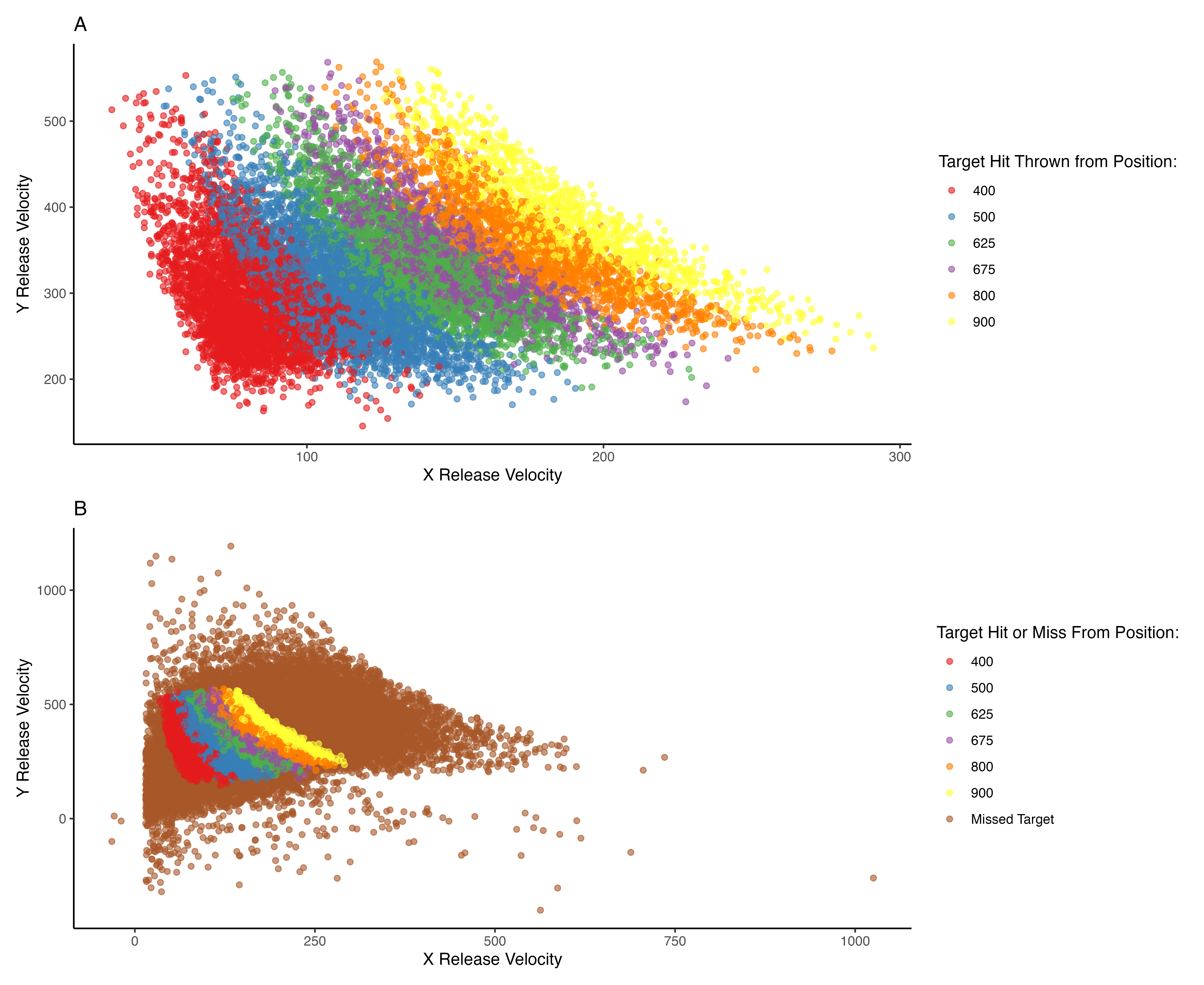
For each individual trial, the Euclidean distance (Equation 1) was computed between the velocity components (x and y) of that trial and the velocity components of each individual solution throw for each of the 6 positions from which participants would be tested in the final phase of the study. The P parameter in Equation 1 is set equal to 2, reflecting a Gaussian similarity gradient. Then, as per an instance-based model of similarity (Logan, 2002; Nosofsky, 1992), these distances were multiplied by a sensitivity parameter, c, and then exponentiated to yield a similarity value. The parameter c controls the rate with which similarity-based generalization drops off as the Euclidean distance between two throws in x- and y-velocity space increases. If c has a large value, then even a small difference between two throws’ velocities greatly decreases the extent of generalization from one to the other. A small value for c produces broad generalization from one throw to another despite relatively large differences in their velocities. The similarity values for each training individual throw made by a given participant were then summed to yield a final similarity score, with a separate score computed for each of the 6 testing positions. The final similarity score is construable as index of how accurate the throws a participant made during the training phase would be for each of the testing positions.
Equation 1: \[ Similarity_{I,J} = \sum_{i=I}\sum_{j=J} (e^{-c^\cdot d^{p}_{i,j}}) \]
Equation 2: \[ d_{i,j} = \sqrt{(x_{Train_i}-x_{Solution_j})^2 + (y_{Train_i}-y_{Solution_j})^2 } \]
A simple linear regression revealed that these similarity scores were significantly predictive of performance in the transfer stage, t =-15.88, p<.01, \(r^2\)=.17, such that greater similarity between training throws and solution spaces for each of the test locations resulted in better performance. We then repeated the group comparisons above while including similarity as a covariate in the model. Comparing the varied and constant groups in testing performance from all testing positions yielded a significant effect of similarity, F(1, 205)=85.66, p<.001, \(\eta^{2}_G\) =.29, and also a significant effect of condition (varied vs. constant), F(1, 205)=6.03, p=.015, \(\eta^{2}_G\) =.03. The group comparison limited to only novel locations for the varied group pit against trained location for the constant group resulted in a significant effect of similarity, F(1,148)=31.12, p<.001, \(\eta^{2}_G\) =.18 as well as for condition F(1,148)=11.55, p<.001, \(\eta^{2}_G\) =.07. For all comparisons, the pattern of results was consistent with the initial findings from Experiment 2, with the varied group still performing significantly better than the constant group.
Fitting model parameters separately by group
To directly control for similarity in Experiment 2, we developed a model-based measure of the similarity between training throws and testing conditions. This similarity measure was a significant predictor of testing performance, e.g., participants whose training throws were more similar to throws that resulted in target hits from the testing positions, tended to perform better during the testing phase. Importantly, the similarity measure did not explain away the group-level benefits of varied training, which remained significant in our linear model predicting testing performance after similarity was added to the model. However, previous research has suggested that participants may differ in their level of generalization as a function of prior experience, and that such differences in generalization gradients can be captured by fitting the generalization parameter of an instance-based model separately to each group (Hahn et al., 2005; Lamberts, 1994). Relatedly, the influential Bayesian generalization model developed by Tenenbaum & Griffiths (2001) predicts that the breadth of generalization will increase when a rational agent encounters a wider variety of examples. Following these leads, we assume that in addition to learning the task itself, participants are also adjusting how generalizable their experience should be. Varied versus constant participants may be expected to learn to generalize their experience to different degrees. To accommodate this difference, the generalization parameter of the instance-based model (in the present case, the \(c\) parameter) can be allowed to vary between the two groups to reflect the tendency of learners to adaptively tune the extent of their generalization. One specific hypothesis is that people adaptively set a value of c to fit the variability of their training experience (Nosofsky & Johansen, 2000; Sakamoto et al., 2006). If one’s training experience is relatively variable, as with the variable training condition, then one might infer that future test situations will also be variable, in which case a low value of c will allow better generalization because generalization will drop off slowly with training-to-testing distance. Conversely, if one’s training experience has little variability, as found in the constant training conditions, then one might adopt a high value of \(c\) so that generalization falls off rapidly away from the trained positions.
To address this possibility, we compared the original instance-based model of similarity fit against a modified model which separately fits the generalization parameter, \(c\), to varied and constant participants. To perform this parameter fitting, we used the optim function in R, and fit the model to find the \(c\) value(s) that maximized the correlation between similarity and testing performance.
Both models generate distinct similarity values between training and testing locations. Much like the analyses in Experiment 2, these similarity values are regressed against testing performance in models of the form shown below. As was the case previously, testing performance is defined as the mean absolute distance from the center of the target (with a separate score for each participant, from each position).
Linear models 1 and 3 both show that similarity is a significant predictor of testing performance (p<.01). Of greater interest is the difference between linear model 2, in which similarity is computed from a single \(c\) value fit from all participants (Similarity1c), with linear model 4, which fits the \(c\) parameter separately between groups (Similarity2c). In linear model 2, the effect of training group remains significant when controlling for Similarity1c (p<.01), with the varied group still performing significantly better. However, in linear model 4 the addition of the Similarity2c predictor results in the effect of training group becoming nonsignificant (p=.40), suggesting that the effect of varied vs. constant training is accounted for by the Similarity2c predictor. Next, to further establish a difference between the models, we performed nested model comparisons using ANOVA, to see if the addition of the training group parameter led to a significant improvement in model performance. In the first comparison, ANOVA(Linear Model 1, Linear Model 2), the addition of the training group predictor significantly improved the performance of the model (F=22.07, p<.01). However, in the second model comparison, ANOVA (Linear model 3, Linear Model 4) found no improvement in model performance with the addition of the training group predictor (F=1.61, p=.20).
Finally, we sought to confirm that similarity values generated from the adjusted Similarity2c model had more predictive power than those generated from the original Similarity1c model. Using the BIC function in R, we compared BIC values between linear model 1 (BIC=14604.00) and linear model 3 (BIC = 14587.64). The lower BIC value of model 3 suggests a modest advantage for predicting performance using a similarity measure computed with two \(c\) values over similarity computed with a single \(c\) value. When fit with separate \(c\) values, the best fitting \(c\) parameters for the model consistently optimized such that the \(c\) value for the varied group (c=.00008) was smaller in magnitude than the \(c\) value for the constant group (c= .00011). Recall that similarity decreases as a Gaussian function of distance (equation 1 above), and a smaller value of \(c\) will result in a more gradual drop-off in similarity as the distance between training throws and testing solutions increases.
In summary, our modeling suggests that an instance-based model which assumes equivalent generalization gradients between constant and varied trained participants is unable to account for the extent of benefits of varied over constant training observed at testing. The evidence for this in the comparative model fits is that when a varied/constant dummy-coded variable for condition is explicitly added to the model, the variable adds a significant contribution to the prediction of test performance, with the variable condition yielding better performance than the constant conditions. However, if the instance-based generalization model is modified to assume that the training groups can differ in the steepness of their generalization gradient, by incorporating a separate generalization parameter for each group, then the instance-based model can account for our experimental results without explicitly taking training group into account. Henceforth this model will be referred to as the Instance-based Generalization with Adaptive Similarity (IGAS) model.
Project 1 General Discussion
Across two experiments, we found evidence in support of the benefits of variability hypothesis in a simple, computerized projectile throwing task. Generalization was observed in both constant and varied participants, in that both groups tended to perform better at novel positions in the testing phase than did participants who started with those positions in the training phase. However, varied trained participants consistently performed better than constant trained participants, in terms of both the testing phase in general, and in a comparison that only included untrained positions. We also found some evidence for the less commonly observed pattern wherein varied-trained participants outperform constant-trained participants even from conditions identical to the constant group training (Goode et al., 2008; Green et al., 1995; Kerr & Booth, 1978). In Experiment 1 varied participants performed significantly better on this identity comparison. In Experiment 2, the comparison was not significant initially, but became significant after controlling for the similarity measure that incorporates only a single value for the steepness of similarity-based generalization (\(c\)). Furthermore, we showed that the general pattern of results from Experiment 2 could be parsimoniously accommodated by an instance-based similarity model, but only with the assumption that constant and varied participants generalize their training experience to different degrees.
Our results thus suggest that the benefits of variation cannot be explained by the varied-trained participants simply covering a broader range of the task space. Rather, the modeling suggests that varied participants also learn to adaptively tune their generalization function such that throwing locations generalize more broadly to one another than they do in the constant condition. A learning system could end up adopting a higher \(c\) value in the constant than variable training conditions by monitoring the trial-by-trial variability of the training items. The \(c\) parameter would be adapted downwards when adjacent training items are dissimilar to each other and adapted upwards when adjacent training items are the same. In this fashion, contextually appropriate \(c\) values could be empirically learned. This learning procedure would capture the insight that if a situation has a high amount variability, then the learner should be predisposed toward thinking that subsequent test items will also show considerable variability, in which case generalization gradients should be broad, as is achieved by low values for \(c\). Sakamoto et al. (2006) implemented a similar learning mechanism for updating the generalization paramater in an exemplar-based model (although in their model, a separate generalization parameter is assigned to each exemplar). In their experiment, participants were trained on a high variability and a low variability category, and the dynamically updated generalization parameter was necessary to account for broader generalization observed around the high variability category when participants were tested with an ambiguous intermediary item. In a subsequent work (Sakamoto et al., 2008), the same authors showed that a similar learning mechanism could account for the pattern wherein participants generalize more broadly around a category when the average distance between the category exemplars is larger (however the only model tested in this work was a prototype model).
Also of interest is whether the IGAS model can predict the pattern of results wherein the varied condition outperforms the constant condition even from the position on which the constant condition trained. Although our models were fit using all of the Experiment 2 training and testing data, not just that of the identity comparisons, in Figure 10 we demonstrate how a simplified version of the IGAS model could in principle produce such a pattern. In addition to the assumption of differential generalization between varied and constant conditions, our simplified model makes explicit an assumption that is incorporated into the full IGAS model – namely that even when being tested from a position identical to that which was trained, there are always some psychological contextual differences between training and testing throws, resulting in a non-zero dissimilarity.
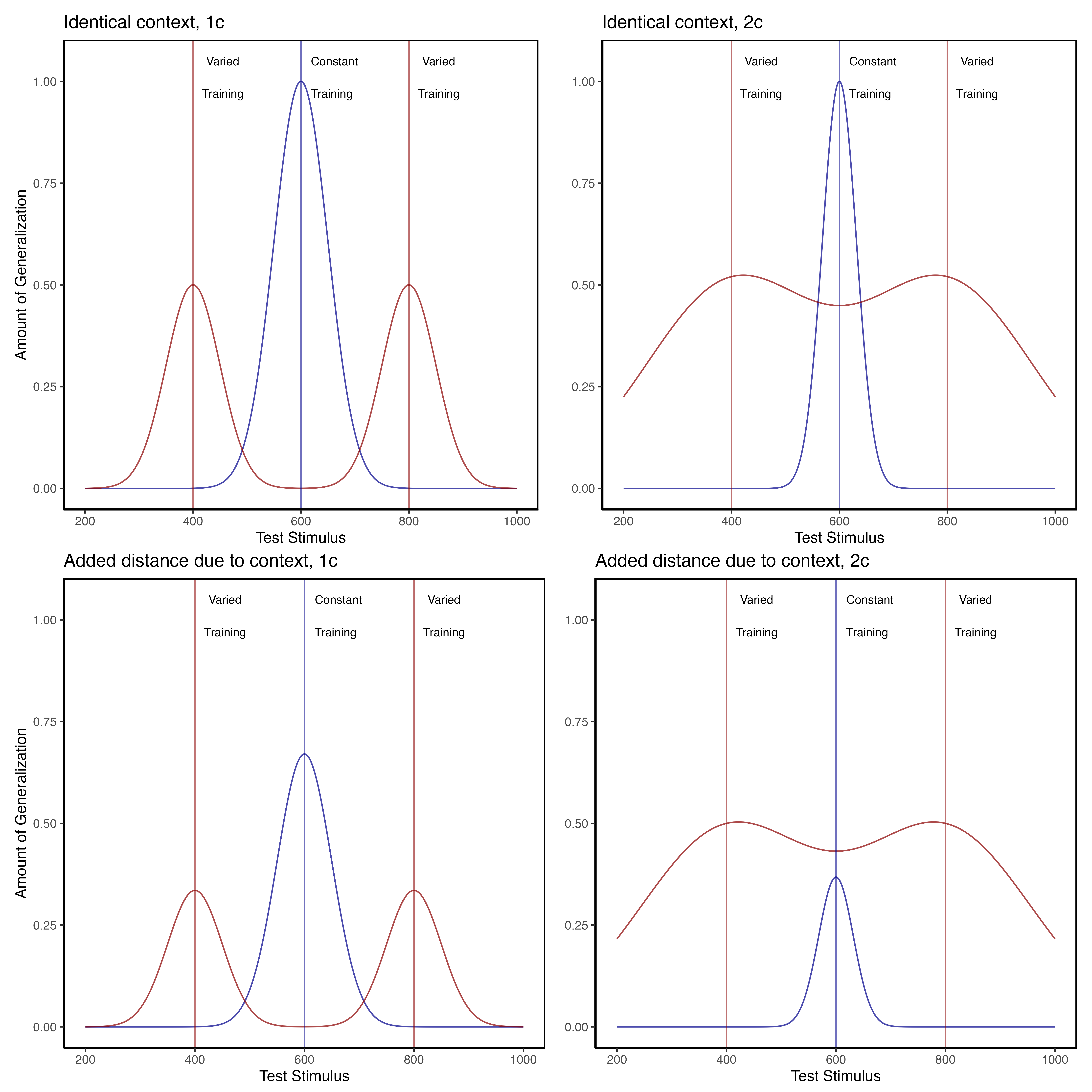
As described above, the idea that learners flexibly adjust their generalization gradient based on prior experience does have precedent in the domains of category learning (Aha & Goldstone, 1992; Briscoe & Feldman, 2011; Hahn et al., 2005; Lamberts, 1994; Op de Beeck et al., 2008), and sensorimotor adaptation (Marongelli & Thoroughman, 2013; Taylor & Ivry, 2013; Thoroughman & Taylor, 2005). Lamberts (1994) showed that a simple manipulation of background knowledge during a categorization test resulted in participants generalizing their training experience more or less broadly, and moreover that such a pattern could be captured by allowing the generalization parameter of an instance-based similarity model to be fit separately between conditions. The flexible generalization parameter has also successfully accounted for generalization behavior in cases where participants have been trained on categories that differ in their relative variability (Hahn et al., 2005; Sakamoto et al., 2006). However, to the best of our knowledge, IGAS is the first instance-based similarity model that has been put forward to account for the effect of varied training in a visuomotor skill task. Although IGAS was inspired by work in the domain of category learning, its success in a distinct domain may not be surprising in light of the numerous prior observations that at least certain aspects of learning and generalization may operate under common principles across different tasks and domains (Censor et al., 2012; Hills et al., 2010; Jamieson et al., 2022; Law & Gold, 2010; Roark et al., 2021; Rosenbaum et al., 2001; Vigo et al., 2018; Wall et al., 2021; Wu et al., 2020; J. Yang et al., 2020).
Our modelling approach does differ from category learning implementations of instance-based models in several ways. One such difference is the nature of the training instances that are assumed to be stored. In category learning studies, instances are represented as points in a multidimensional space of all of the attributes that define a category item (e.g., size/color/shape). Rather than defining instances in terms of what stimuli learners experience, our approach assumes that stored, motor instances reflect how they act, in terms of the velocity applied to the ball on each throw. An advantage of many motor learning tasks is the relative ease with which task execution variables can be directly measured (e.g., movement force, velocity, angle, posture) in addition to the decision and response time measures that typically exhaust the data generated from more classical cognitive tasks. Of course, whether learners actually are storing each individual motor instance is a fundamental question beyond the scope of the current work – though as described in the introduction there is some evidence in support of this idea (Chamberlin & Magill, 1992a; Crump & Logan, 2010; Hommel, 1998; Meigh et al., 2018; Poldrack et al., 1999). A particularly noteworthy instance-based model of sensory-motor behavior is the Knowledge II model of Rosenbaum and colleagues (R. G. Cohen & Rosenbaum, 2004; Rosenbaum et al., 1995). Knowledge II explicitly defines instances as postures (joint combinations), and is thus far more detailed than IGAS in regards to the contents of stored instances. Knowledge II also differs from IGAS in that learning is accounted for by both the retrieval of stored postures, and the generation of novel postures via the modification of retrieved postures. A promising avenue for future research would be to combine the adaptive similarity mechanism of IGAS with the novel instance generation mechanisms of Knowledge II.
Our findings also have some conceptual overlap with an earlier study on the effects of varied training in a coincident timing task (Catalano & Kleiner, 1984). In this task, participants observe a series of lamps lighting up consecutively, and attempt to time a button press with the onset of the final lamp. The design consisted of four separate constant groups, each training from a single lighting velocity, and a single varied group training with all four of the lighting velocities used by the individual constant groups. Participants were then split into four separate testing conditions, each of which were tested from a single novel lighting velocity of varying distance from the training conditions. The result of primary interest was that all participants performed worse as the distance between training and testing velocity increased – a typical generalization decrement. However, varied participants showed less of a decrement than did constant participants. The authors take this result as evidence that varied training results in a less-steep generalization gradient than does constant training. Although the experimental conclusions of Catalano and Kleiner are similar to our own, our work is novel in that we account for our results with a cognitive model, and without assuming the formation of a schema. Additionally, the way in which Catalano and Kleiner collapse their separate constant groups together may result in similarity confounds between varied and constant conditions that leaves their study open to methodological criticisms, especially in light of related work which demonstrated that the extent to which varied training may be beneficial can depend on whether the constant group they are compared against trained from similar conditions to those later tested (Wrisberg et al., 1987). Our study alleviates such concerns by explicitly controlling for similarity.
Limitations
A limitation of this study concerns the ordering of the testing/transfer trials at the conclusion of both experiments. Participants were tested from each separate position (4 in Experiment 1, 6 in Experiment 2) in a random, intermixed order. Because the varied group was trained from two positions that were also randomly ordered, they may have benefited from experience with this type of sequencing, whereas the constant groups had no experience with switching between positions trial to trial. This concern is somewhat ameliorated by the fact that the testing phase performance of the constant groups from their trained position was not significantly worse than their level of performance at the end of the training phase, suggesting that they were not harmed by random ordering of positions during testing. It should also be noted that the computerized task utilized in the present work is relatively simple compared to many of the real-world tasks utilized in prior research. It is thus conceivable that the effect of variability in more complex tasks is distinct from the process put forward in the present work. An important challenge for future work will be to assess the extent to which IGAS can account for generalization in relatively complex tasks with far more degrees of freedom.
It is common for psychological process models of categorization learning to use an approach such as multidimensional scaling so as to transform the stimuli from the physical dimensions used in the particular task into the psychological dimensions more reflective of the actual human representations (Nosofsky, 1992; Shepard, 1987). Such scaling typically entails having participants rate the similarity between individual items and using these similarity judgements to then compute the psychological distances between stimuli, which can then be fed into a subsequent model. In the present investigation, there was no such way to scale the x and y velocity components in terms of the psychological similarity, and thus our modelling does rely on the assumption that the psychological distances between the different throwing positions are proportional to absolute distances in the metric space of the task (e.g., the relative distance between positions 400 and 500 is equivalent to that between 800 and 900). However, an advantage of our approach is that we are measuring similarity in terms of how participants behave (applying a velocity to the ball), rather than the metric features of the task stimuli.
Conclusion
Our experiments demonstrate a reliable benefit of varied training in a simple projectile launching task. Such results were accounted for by an instance-based model that assumes that varied training results in the computation of a broader similarity-based generalization gradient. Instance-based models augmented with this assumption may be a valuable approach towards better understanding skill generalization and transfer.
Project 2
Introduction
A longstanding issue across both science and instruction has been to understand how various aspects of an educational curriculum or training program influence learning acquisition and generalization. One such aspect, which has received a great deal of research attention, is the variability of examples experienced during training (Raviv et al., 2022). The influence of training variation has been studied in numerous domains, including category learning (A. L. Cohen et al., 2001; Posner & Keele, 1968), visuomotor learning (Berniker et al., 2014; Schmidt, 1975), language learning (Perry et al., 2010), and education (Braithwaite & Goldstone, 2015; Guo et al., 2014). The pattern of results is complex, with numerous studies finding both beneficial (Braun et al., 2009; Catalano & Kleiner, 1984; Gorman & Goldstone, 2022; Roller et al., 2001), as well as null or negative effects (Brekelmans et al., 2022; Hu & Nosofsky, 2024; Van Rossum, 1990). The present study seeks to contribute to the large body of existing research by examining the influence of variability in visuomotor function learning - a domain in which it has been relatively under-studied.
Function Learning and Extrapolation
The study of human function learning investigates how people learn relationships between continuous input and output values. Function learning is studied both in tasks where individuals are exposed to a sequence of input/output pairs (DeLosh et al., 1997; McDaniel et al., 2013), or situations where observers are presented with an incomplete scatterplot or line graph and make predictions about regions of the plot that do not contain data (Ciccione & Dehaene, 2021; Courrieu, 2012; Said & Fischer, 2021; Schulz et al., 2020). Studies of function learning often compare the difficulty of learning functions of different underlying forms (e.g. linear, bi-linear, power, sinusoidal), and the extent to which participants can accurately respond to novel inputs that fall in-between previously experienced inputs (interpolation testing), or that fall outside the range of previously experienced inputs (extrapolation).
Carroll (1963) conducted the earliest work on function learning. Input stimuli and output responses were both lines of varying length. The correct output response was related to the length of the input line by a linear, quadratic, or random function. Participants in the linear and quadratic performed above chance levels during extrapolation testing, with those in the linear condition performing the best overall. Carroll argued that these results were best explained by a rule-based model wherein learners form an abstract representation of the underlying function. Subsequent work by Brehmer (1974), testing a wider array of functional forms, provided further evidence for superior extrapolation in tasks with linear functions. Brehmer argued that individuals start out assuming a linear function, but given sufficient error will progressively test alternative hypotheses with polynomials of greater degree. Koh & Meyer (1991) employed a visuomotor function learning task, wherein participants were trained on examples from an unknown function relating the length of an input line to the duration of a response (time between keystrokes). In this domain, participants performed best when the relation between line length and response duration was determined by a power law, as opposed to linear function. Koh and Meyer developed the log-polynomial adaptive-regression model to account for their results.
The first significant challenge to rule-based accounts of function learning was put forth by DeLosh et al. (1997) . In their task, participants learned to associate stimulus magnitudes with response magnitudes that were related via either linear, exponential, or quadratic function. Participants approached ceiling performance by the end of training in each function condition, and were able to accurately respond on interpolation testing trials. All three conditions demonstrated some capacity for extrapolation, however participants in the linear condition tended to underestimate the true function, while exponential and quadratic participants reliably overestimated the true function on extrapolation trials. Extrapolation and interpolation performances are depicted in Figure 11.
The authors evaluated the rule-based models introduced in earlier research (with some modifications enabling trial-by-trial learning). The polynomial hypothesis testing model (Brehmer, 1974; Carroll, 1963) tended to mimic the true function closely in extrapolation, and thus offered a poor account of the under and over-estimation biases shown in the human data. The log-polynomial adaptive regression model (Koh & Meyer, 1991) was able to mimic some of the systematic deviations produced by human subjects, but also predicted overestimation in cases where underestimation occurred.
The authors also introduced two new function-learning models. The Associative Learning Model (ALM) and the extrapolation-association model (EXAM). ALM is a two-layer connectionist model adapted from the ALCOVE model in the category learning literature (Kruschke, 1992). ALM belongs to the general class of radial-basis function neural networks, and can be considered a similarity-based model in the sense that the nodes in the input layer of the network are activated as a function of distance (see Figure 27). The EXAM model retains the same similarity-based activation and associative learning mechanisms as ALM, while being augmented with a linear rule response mechanism. When presented with novel stimuli, EXAM will retrieve the most similar input-output examples encountered during training, and from those examples compute a local slope. ALM was able to provide a good account of participants’ training and interpolation data in all three function conditions, however it was unable to extrapolate. EXAM, by contrast, was able to reproduce both the extrapolation underestimation, as well as the quadratic and exponential overestimation patterns exhibited by the human participants. Subsequent research identified some limitations in EXAM’s ability to account for cases where human participants learn and extrapolate a sinusoidal function (Bott & Heit, 2004) or to scenarios where different functions apply to different regions of the input space (Kalish et al., 2004), though EXAM has been shown to provide a good account of human learning and extrapolation in tasks with bi-linear, V-shaped input spaces (McDaniel et al., 2009).

Variability and Function Learning
The influence of variability on function learning tasks has received relatively little attention. The study by DeLosh et al. (1997) (described in detail above) did include a variability manipulation (referred to as density in their paper), wherein participants were trained with either 8, 20, or 50 unique input-output pairs, with the total number of training trials held constant. They found a minimal influence of variability on training performance, and no difference between groups in interpolation or extrapolation, with all three variability conditions displaying accurate interpolation, and linearly biased extrapolation that was well accounted for by the EXAM model.
In the domain of visuomotor learning, van Dam & Ernst (2015) employed a task which required participants to learn a linear function between the spikiness of shape stimuli and the correct horizontal position to make a rapid pointing response. The shapes ranged from very spiky to completely circular at the extreme ends of the space. Participants trained with intermediate shapes having lower variation (2 shapes) or higher variation (5 shapes) condition, with the 2 items of the lower variation condition matching the items used on the extreme ends of the higher variation training space. Learning was significantly slower in the higher variation group. However, the two conditions did not differ when tested with novel shapes, with both groups producing extrapolation responses of comparable magnitude to the most similar training item, rather than in accordance with the true linear function. The authors accounted for both learning and extrapolation performance with a Bayesian learning model. Similar to ALM, the model assumes that generalization occurs as a Gaussian function of the distance between stimuli. However, unlike ALM, the Bayesian learning model utilizes more elaborate probabilistic stimulus representations, with a separate Kalman Filter for each shape stimulus.
Overview Of Present Study
The present study investigates the influence of training variability on learning, generalization, and extrapolation in a uni-dimensional visuomotor function learning task. To the best of our knowledge, this research is the first to employ the classic constant vs. varied training manipulation, commonly used in the literature studying the benefits of variability, in the context of a uni-dimensional function learning task. Across three experiments, we compare constant and varied training conditions in terms of learning performance, extrapolation accuracy, and the ability to reliably discriminate between stimuli.
To account for the empirical results, we will apply a series of computational models, including the Associative Learning Model (ALM) and the Extrapolation-Association Model (EXAM). Notably, this study is the first to employ approximate Bayesian computation (ABC) to fit these models to individual subject data, enabling us to thoroughly investigate the full range of posterior predictions of each model, and to examine the ability of these influential models of function learning to account for both the group level and individual level data.
Experiment 1
Methods
Participants. A total of 183 participants were initially recruited from Indiana University Introductory Psychology Courses. Of these, 27 participants were excluded from further analysis due to meeting the exclusion criteria, resulting in a final sample of 156 participants. The exclusion criteria was defined as performance worse (i.e., larger deviations) than the condition average in either the training or testing stage of the experiment. The remaining participants were randomly assigned to one of two training conditions: varied training or constant training.
Task. The “Hit The Wall” (HTW) visuomotor extrapolation task was programmed in JavaScript, making use of the phaser.io game library. The HTW task involved launching a projectile such that it would strike the “wall” at the target speed indicated at the top of the screen (see Figure 12). The target velocities were given as a range, or band, of acceptable velocity values (e.g., band 800-1000). During the training stage, participants received feedback indicating whether they had hit the wall within the target velocity band, or how many units their throw was above or below the target band. Participants were instructed that only the x velocity component of the ball was relevant to the task. The y velocity, or the location at which the ball struck the wall, had no influence on the task feedback.

Procedure. All participants completed the task online. Participants were provided with a description of the experiment and indicated informed consent. Figure 13 illustrates the general procedure. Participants completed a total of 90 trials during the training stage. In the varied training condition, participants encountered three velocity bands (800-1000, 1000-1200, and 1200-1400). Participants in the constant training condition trained on only one velocity band (800-1000) - the closest band to what would be the novel extrapolation bands in the testing stage.
Following the training stage, participants proceeded immediately to the testing stage. Participants were tested from all six velocity bands, in two separate stages. In the novel extrapolation testing stage, participants completed “no-feedback” testing from three novel extrapolation bands (100-300, 350-550, and 600-800), with each band consisting of 15 trials. Participants were also tested from the three velocity bands that were trained by the varied condition (800-1000, 1000-1200, and 1200-1400). In the constant training condition, two of these bands were novel, while in the varied training condition, all three bands were encountered during training. The order in which participants completed the novel-extrapolation and testing-from-3-varied bands was counterbalanced across participants. A final training stage presented participants with “feedback” testing for each of the three extrapolation bands (100-300, 350-550, and 600-800).
Analyses Strategy
All data processing and statistical analyses were performed in R version 4.32 (Team, 2020). To assess differences between groups, we used Bayesian Mixed Effects Regression. Model fitting was performed with the brms package in R (Bürkner, 2017), and descriptive stats and tables were extracted with the BayestestR package (Makowski et al., 2019). Mixed effects regression enables us to take advantage of partial pooling, simultaneously estimating parameters at the individual and group level. Our use of Bayesian, rather than frequentist methods allows us to directly quantify the uncertainty in our parameter estimates, as well as avoid convergence issues common to the frequentist analogues of our mixed models.
Each model was set to run with 4 chains, 5000 iterations per chain, with the first 2500 discarded as warmup chains. Rhat values were within an acceptable range, with values <=1.02 (see appendix for diagnostic plots). We used uninformative priors for the fixed effects of the model (condition and velocity band), and weakly informative Student T distributions for the random effects. For each model, we report 1) the mean values of the posterior distribution for the parameters of interest, 2) the lower and upper credible intervals (CrI), and the probability of direction value (pd).
| Group Comparison | Code | Data |
|---|---|---|
| End of Training Accuracy | brm(Abs. Deviation ~ condit) |
Final Training Block |
| Test Accuracy | brm(Abs. Deviation ~ condit * bandType + (1|id) + (1|bandInt) |
All Testing trials |
| Band Discrimination | brm(vx ~ condit * band +(1 + bandInt|id) |
All Testing Trials |
In each experiment we compare varied and constant conditions in terms of 1) accuracy in the final training block; 2) testing accuracy as a function of band type (trained vs. extrapolation bands); 3) extent of discrimination between all six testing bands. We quantified accuracy as the absolute deviation between the response velocity and the nearest boundary of the target band. Thus, when the target band was velocity 600-800, throws of 400, 650, and 900 would result in deviation values of 200, 0, and 100, respectively. The degree of discrimination between bands was measured by fitting a linear model predicting the response velocity as a function of the target velocity. Participants who reliably discriminated between velocity bands tended to have slope values ~1, while participants who made throws irrespective of the current target band would have slopes ~0.
Results
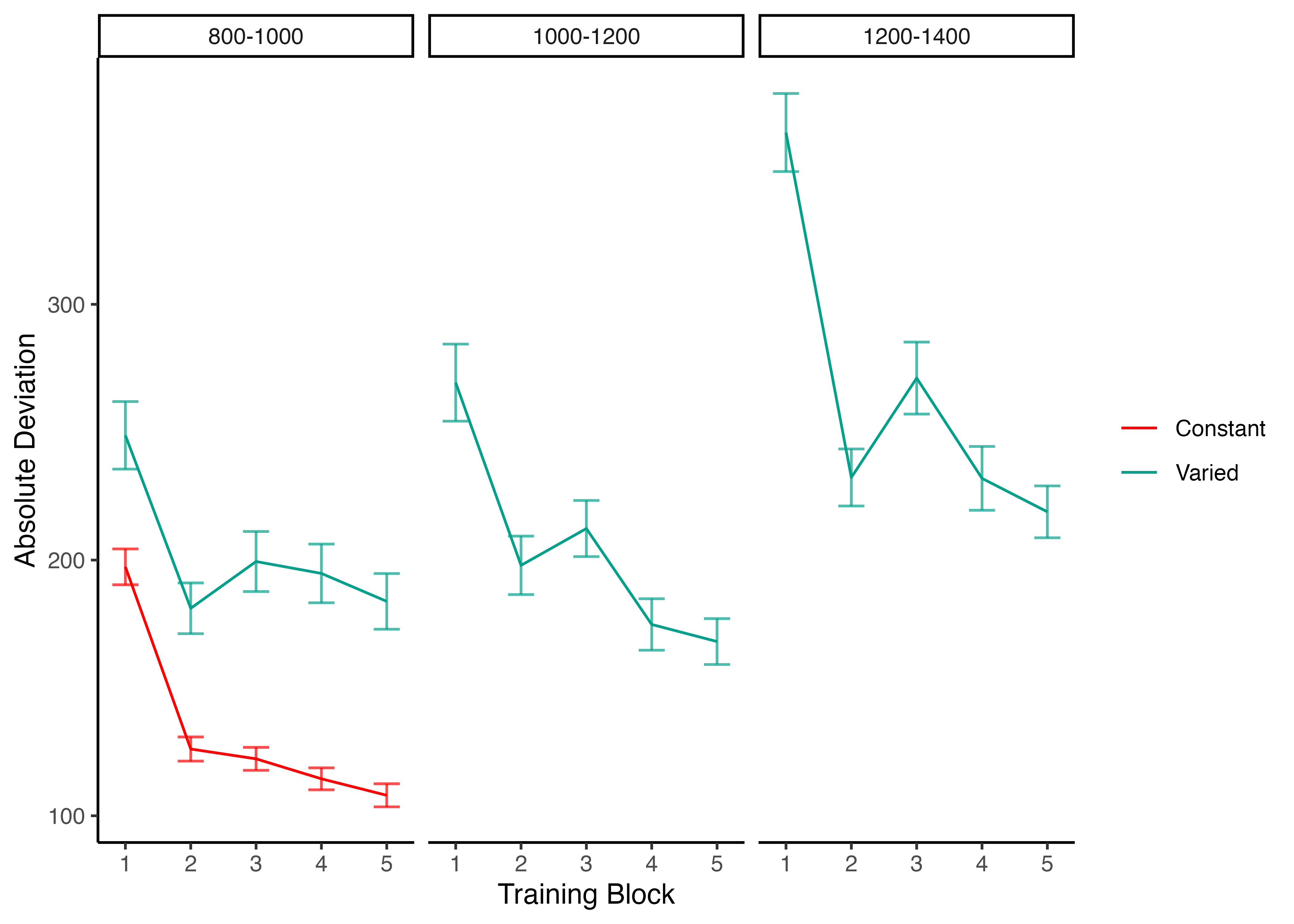
| Term | Estimate | 95% CrI Lower | 95% CrI Upper | pd |
|---|---|---|---|---|
| Intercept | 106.34 | 95.46 | 117.25 | 1 |
| conditVaried | 79.64 | 57.92 | 101.63 | 1 |
Training. Figure 14 displays the average deviations across training blocks for the varied group, which trained on three velocity bands, and the constant group, which trained on one velocity band. To compare the training conditions at the end of training, we analyzed performance on the 800-1000 velocity band, which both groups trained on. The full model results are shown in Table 1. The varied group had a significantly greater deviation from the target band than the constant group in the final training block, (\(\beta\) = 79.64, 95% CrI [57.92, 101.63]; pd = 100%).
| Term | Estimate | 95% CrI Lower | 95% CrI Upper | pd |
|---|---|---|---|---|
| Intercept | 152.55 | 70.63 | 229.85 | 1.0 |
| conditVaried | 39.00 | -21.10 | 100.81 | 0.9 |
| bandTypeExtrapolation | 71.51 | 33.24 | 109.60 | 1.0 |
| conditVaried:bandTypeExtrapolation | 66.46 | 32.76 | 99.36 | 1.0 |
Testing. To compare accuracy between groups in the testing stage, we fit a Bayesian mixed effects model predicting deviation from the target band as a function of training condition (varied vs. constant) and band type (trained vs. extrapolation), with random intercepts for participants and bands. The model results are shown in Table 7. The main effect of training condition was not significant (\(\beta\) = 39, 95% CrI [-21.1, 100.81]; pd = 89.93%). The extrapolation testing items had a significantly greater deviation than the training bands (\(\beta\) = 71.51, 95% CrI [33.24, 109.6]; pd = 99.99%). Most importantly, the interaction between training condition and band type was significant (\(\beta\) = 66.46, 95% CrI [32.76, 99.36]; pd = 99.99%), As shown in Figure 15, the varied group had disproportionately larger deviations compared to the constant group in the extrapolation bands.
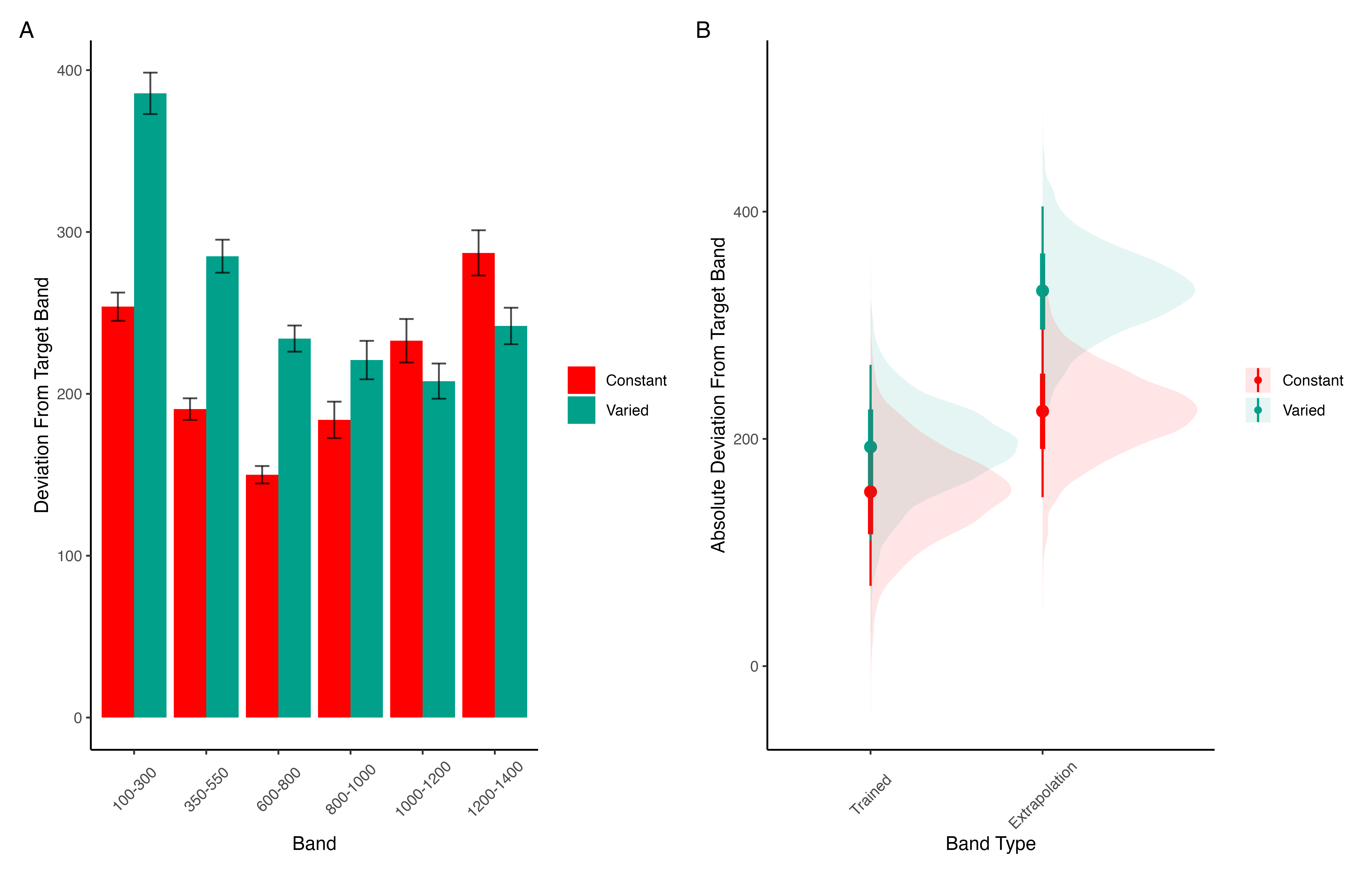
| Term | Estimate | 95% CrI Lower | 95% CrI Upper | pd |
|---|---|---|---|---|
| Intercept | 408.55 | 327.00 | 490.61 | 1.00 |
| conditVaried | 164.05 | 45.50 | 278.85 | 1.00 |
| Band | 0.71 | 0.62 | 0.80 | 1.00 |
| condit*Band | -0.14 | -0.26 | -0.01 | 0.98 |
Finally, to assess the ability of both conditions to discriminate between velocity bands, we fit a model predicting velocity as a function of training condition and velocity band, with random intercepts and random slopes for each participant. See Table 8 for the full model results. The estimated coefficient for training condition (\(\beta\) = 164.05, 95% CrI [45.5, 278.85], pd = 99.61%) suggests that the varied group tends to produce harder throws than the constant group, though this is not, in and of itself, useful for assessing discrimination. Most relevant to the issue of discrimination is the coefficient on the Band predictor (\(\beta\) = 0.71 95% CrI [0.62, 0.8], pd = 100%). Although the median slope does fall underneath the ideal of value of 1, the fact that the 95% credible interval does not contain 0 provides strong evidence that participants exhibited some discrimination between bands. The significant negative estimate for the interaction between slope and condition (\(\beta\) = -0.14, 95% CrI [-0.26, -0.01], pd = 98.39%), indicates that the discrimination was modulated by training condition, with the varied participants showing less sensitivity between bands than the constant condition (see Figure 16 and Figure 17).

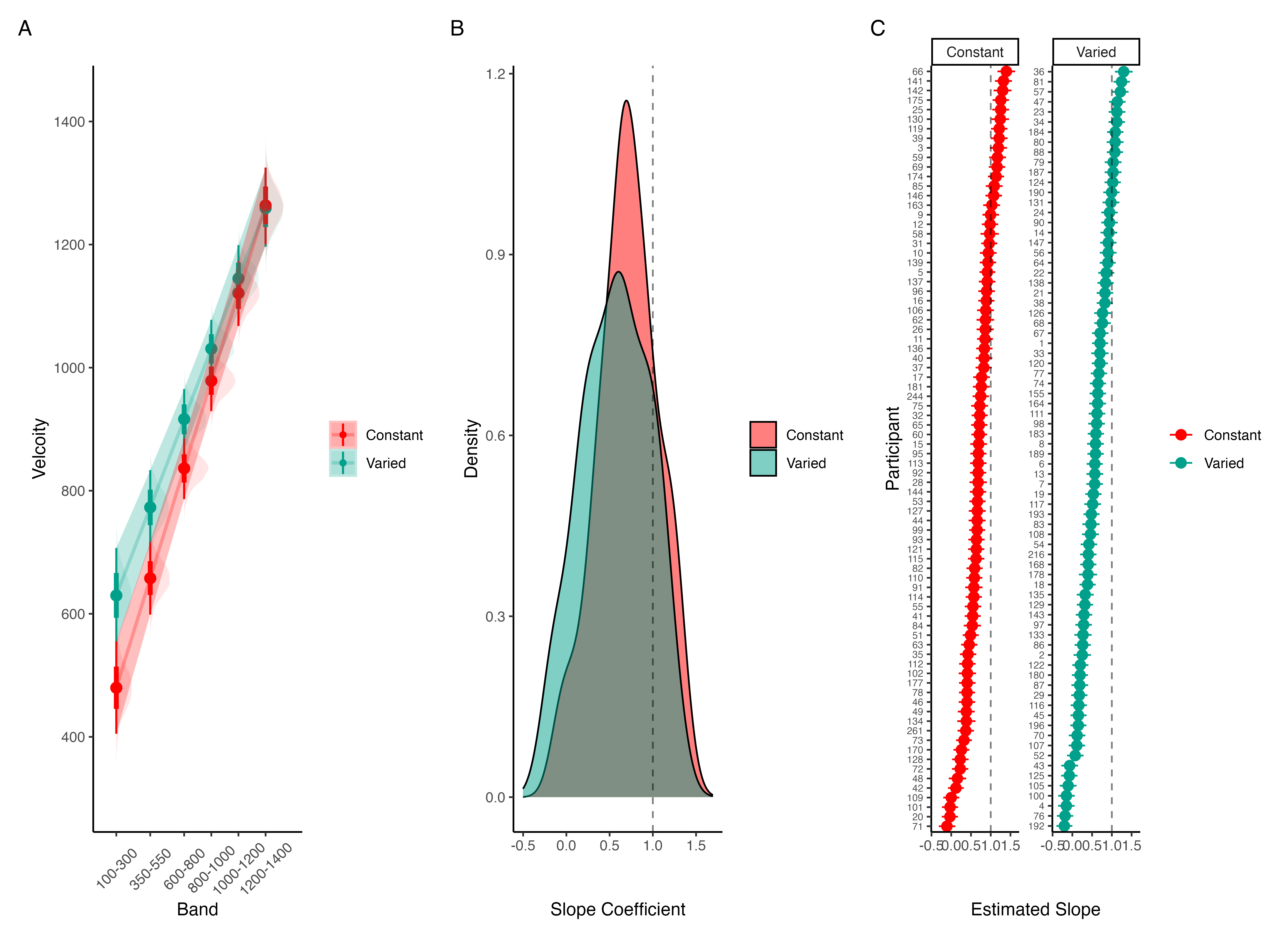
Experiment 1 Summary
In Experiment 1, we investigated how variability in training influenced participants’ ability to learn and extrapolate in a visuomotor task. Our findings that training with variable conditions resulted in lower final training performance are consistent with much of the prior research on the influence of training variability (Raviv et al., 2022; Soderstrom & Bjork, 2015), and are particularly unsurprising in the present work, given that the constant group received three times the amount of training on the velocity band common to the two conditions.
More importantly, the varied training group exhibited significantly larger deviations from the target velocity bands during the testing phase, particularly for the extrapolation bands that were not encountered by either condition during training.
Experiment 2
Methods & Procedure
Initially, 131 participants were recruited. After applying the same exclusion procedure as in Experiment 1, 21 participants were excluded, resulting in a final sample of 110 participants who completed the experiment (Varied: 55, Constant: 55). The task and procedure of Experiment 2 was identical to Experiment 1, with the exception that the training and testing bands were reversed (see Figure 18). The Varied group trained on bands 100-300, 350-550, 600-800, and the constant group trained on band 600-800. Both groups were tested from all six bands.
Results

| Term | Estimate | 95% CrI Lower | 95% CrI Upper | pd |
|---|---|---|---|---|
| Intercept | 91.01 | 80.67 | 101.26 | 1 |
| conditVaried | 36.15 | 16.35 | 55.67 | 1 |
Training. Figure 19 presents the deviations across training blocks for both constant and varied training groups. We again compared training performance on the band common to both groups (600-800). The full model results are shown in Table 1. The varied group had a significantly greater deviation than the constant group in the final training block, ( \(\beta\) = 36.15, 95% CrI [16.35, 55.67]; pd = 99.95%).
| Term | Estimate | 95% CrI Lower | 95% CrI Upper | pd |
|---|---|---|---|---|
| Intercept | 190.91 | 125.03 | 259.31 | 1.00 |
| conditVaried | -20.58 | -72.94 | 33.08 | 0.78 |
| bandTypeExtrapolation | 38.09 | -6.94 | 83.63 | 0.95 |
| conditVaried:bandTypeExtrapolation | 82.00 | 41.89 | 121.31 | 1.00 |
Testing Accuracy. The analysis of testing accuracy examined deviations from the target band as influenced by training condition (Varied vs. Constant) and band type (training vs. extrapolation bands). The results, summarized in Table 10, reveal no significant main effect of training condition (\(\beta\) = -20.58, 95% CrI [-72.94, 33.08]; pd = 77.81%). However, the interaction between training condition and band type was significant (\(\beta\) = 82, 95% CrI [41.89, 121.31]; pd = 100%), with the varied group showing disproportionately larger deviations compared to the constant group on the extrapolation bands (see Figure 20).
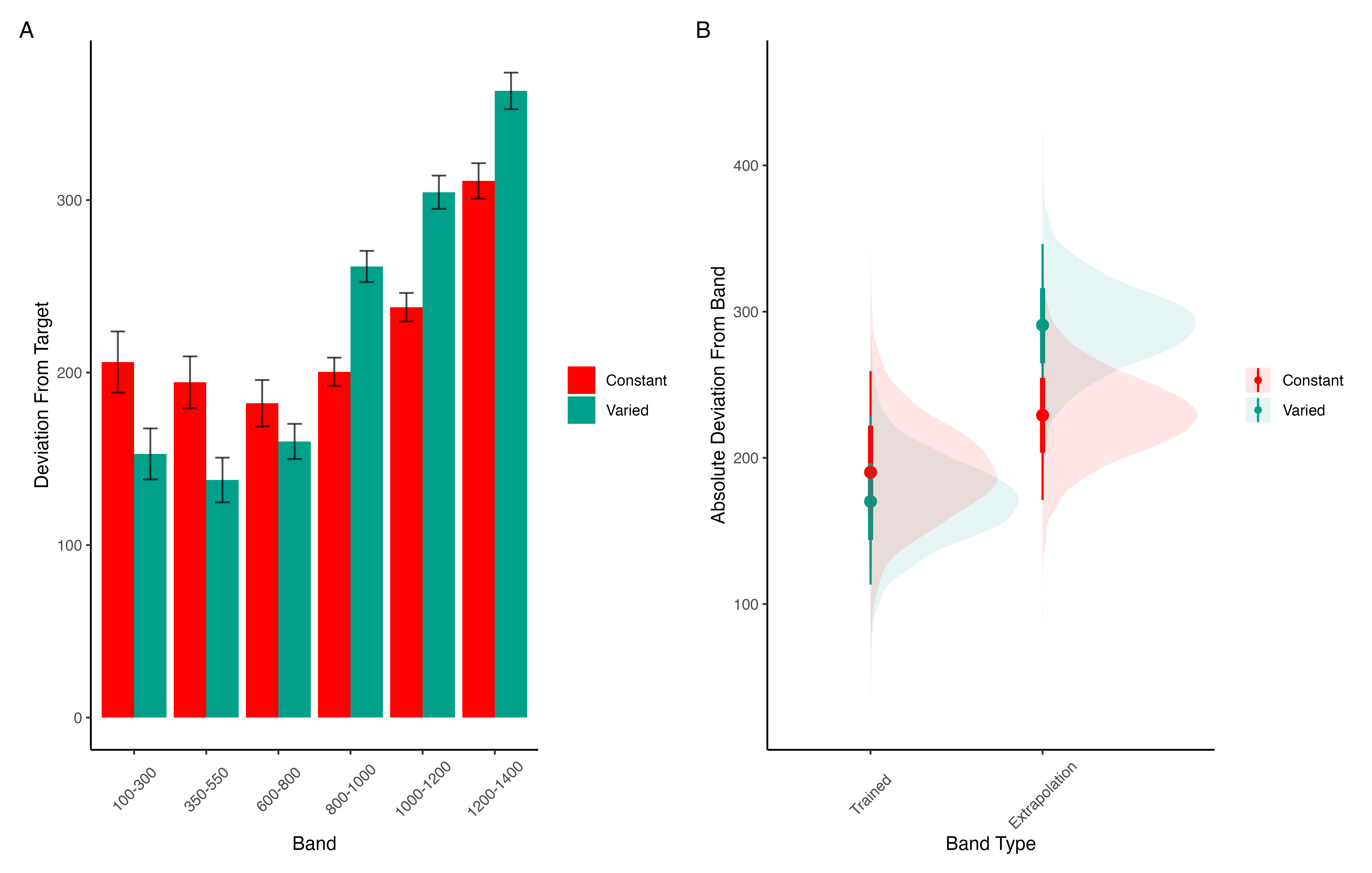
| Term | Estimate | 95% CrI Lower | 95% CrI Upper | pd |
|---|---|---|---|---|
| Intercept | 362.64 | 274.85 | 450.02 | 1.00 |
| conditVaried | -8.56 | -133.97 | 113.98 | 0.55 |
| Band | 0.71 | 0.58 | 0.84 | 1.00 |
| condit*Band | -0.06 | -0.24 | 0.13 | 0.73 |
Testing Discrimination. Finally, to assess the ability of both conditions to discriminate between velocity bands, we fit a model predicting velocity as a function of training condition and velocity band, with random intercepts and random slopes for each participant. The full model results are shown in Table 11. The overall slope on target velocity band predictor was significantly positive, (\(\beta\) = 0.71, 95% CrI [0.58, 0.84]; pd= 100%), indicating that participants exhibited discrimination between bands. The interaction between slope and condition was not significant, (\(\beta\) = -0.06, 95% CrI [-0.24, 0.13]; pd= 72.67%), suggesting that the two conditions did not differ in their ability to discriminate between bands (see Figure 21 and Figure 22).
Experiment 2 Summary
Experiment 2 extended the findings of Experiment 1 by examining the effects of training variability on extrapolation performance in a visuomotor function learning task, but with reversed training and testing bands. Similar to Experiment 1, the Varied group exhibited poorer performance during training and testing. However, unlike experiment 1, the Varied and Constant groups did not show a significant difference in their discrimination between bands.
Experiment 3
In Experiment 3, we sought to further explore the generality of the findings from the first two experiments by modifying the type of feedback provided during training. Specifically, we provided ordinal feedback instead of the continuous feedback used in the previous two experiments. Ordinal feedback provides learners with directional information about the results of their throw (e.g., above the target, below the target, or hitting the target) rather than precise numerical deviations. This form of feedback resembles many real-world learning scenarios, such as a coach instructing an athlete to perform a movement using “more force” or “less force”, or a teacher providing letter grades rather than numeric scores. Although ordinal feedback provides less detailed information per trial, prior research has shown that less detailed feedback is not necessarily detrimental to learning. For example, Cornwall et al. (2022) manipulated whether participants received categorical (correct or incorrect) vs. numerical feedback (reward points ranging from 50-100). They found that the categorical condition produced superior learning, which they explained as arising from larger prediction errors. While we do not make specific predictions about the ordinal condition, this manipulation allows us to explore how different types of feedback might interact with training variability to influence learning and generalization.
Methods & Procedure
The only adjustment of Experiment 3 is for participants to receive ordinal feedback during training, in contrast to the continuous feedback of the prior experiments. After each training throw, participants are informed whether a throw was too soft, too hard, or correct (i.e. within the target velocity range). All other aspects of the task and design are identical to Experiments 1 and 2. We utilized the order of training and testing bands from both of the prior experiments, thus assigning participants to both an order condition (Original or Reverse) and a training condition (Constant or Varied). Participants were once again recruited from the online Indiana University Introductory Psychology Course pool. Following exclusions, 195 participants were included in the final analysis, n=51 in the Constant-Original condition, n=59 in the Constant-Reverse condition, n=39 in the Varied-Original condition, and n=46 in the Varied-Reverse condition.
Results
| Term | Estimate | 95% CrI Lower | 95% CrI Upper | pd |
|---|---|---|---|---|
| Intercept | 121.86 | 109.24 | 134.60 | 1.00 |
| conditVaried | 64.93 | 36.99 | 90.80 | 1.00 |
| bandOrderReverse | 1.11 | -16.02 | 18.16 | 0.55 |
| conditVaried:bandOrderReverse | -77.02 | -114.16 | -39.61 | 1.00 |
Training. Figure 23 displays the average deviations from the target band across training blocks, and Table 12 shows the results of the Bayesian regression model predicting the deviation from the common band at the end of training (600-800 for reversed order, and 800-1000 for original order conditions). The main effect of training condition is significant, with the varied condition showing larger deviations ( \(\beta\) = 64.93, 95% CrI [36.99, 90.8]; pd = 100%). The main effect of band order is not significant \(\beta\) = 1.11, 95% CrI [-16.02, 18.16]; pd = 55.4%, however the interaction between training condition and band order is significant, with the varied condition showing greater accuracy in the reverse order condition ( \(\beta\) = -77.02, 95% CrI [-114.16, -39.61]; pd = 100%).

| Term | Estimate | 95% CrI Lower | 95% CrI Upper | pd |
|---|---|---|---|---|
| Intercept | 288.65 | 199.45 | 374.07 | 1.00 |
| conditVaried | -40.19 | -104.68 | 23.13 | 0.89 |
| bandTypeExtrapolation | -23.35 | -57.28 | 10.35 | 0.92 |
| bandOrderReverse | -73.72 | -136.69 | -11.07 | 0.99 |
| conditVaried:bandTypeExtrapolation | 52.66 | 14.16 | 90.23 | 1.00 |
| conditVaried:bandOrderReverse | -37.48 | -123.28 | 49.37 | 0.80 |
| bandTypeExtrapolation:bandOrderReverse | 80.69 | 30.01 | 130.93 | 1.00 |
| conditVaried:bandTypeExtrapolation:bandOrder | 30.42 | -21.00 | 81.65 | 0.87 |
Testing Accuracy. Table 13 presents the results of the Bayesian mixed effects model predicting absolute deviation from the target band during the testing stage. There was no significant main effect of training condition,\(\beta\) = -40.19, 95% CrI [-104.68, 23.13]; pd = 89.31%, or band type,\(\beta\) = -23.35, 95% CrI [-57.28, 10.35]; pd = 91.52%. However the effect of band order was significant, with the reverse order condition showing lower deviations, \(\beta\) = -73.72, 95% CrI [-136.69, -11.07]; pd = 98.89%. The interaction between training condition and band type was also significant \(\beta\) = 52.66, 95% CrI [14.16, 90.23]; pd = 99.59%, with the varied condition showing disproprionately large deviations on the extrapolation bands compared to the constant group. There was also a significant interaction between band type and band order, \(\beta\) = 80.69, 95% CrI [30.01, 130.93]; pd = 99.89%, such that the reverse order condition showed larger deviations on the extrapolation bands. No other interactions were significant.
| Term | Estimate | 95% CrI Lower | 95% CrI Upper | pd |
|---|---|---|---|---|
| Intercept | 601.83 | 504.75 | 699.42 | 1.00 |
| conditVaried | 12.18 | -134.94 | 162.78 | 0.56 |
| bandOrderReverse | 13.03 | -123.89 | 144.67 | 0.58 |
| Band | 0.49 | 0.36 | 0.62 | 1.00 |
| conditVaried:bandOrderReverse | -338.15 | -541.44 | -132.58 | 1.00 |
| conditVaried:Band | -0.04 | -0.23 | 0.15 | 0.67 |
| bandOrderReverse:band | -0.10 | -0.27 | 0.08 | 0.86 |
| conditVaried:bandOrderReverse:band | 0.42 | 0.17 | 0.70 | 1.00 |
Testing Discrimination. The full results of the discrimination model are presented in Table 13. For the purposes of assessing group differences in discrimination, only the coefficients including the band variable are of interest. The baseline effect of band represents the slope coefficient for the constant training - original order condition, this effect was significant \(\beta\) = 0.49, 95% CrI [0.36, 0.62]; pd = 100%. Neither of the two way interactions reached significance, \(\beta\) = -0.04, 95% CrI [-0.23, 0.15]; pd = 66.63%, \(\beta\) = -0.1, 95% CrI [-0.27, 0.08]; pd = 86.35%. However, the three way interaction between training condition, band order, and target band was significant, \(\beta\) = 0.42, 95% CrI [0.17, 0.7]; pd = 99.96% - indicating a greater slope for the varied condition trained with reverse order bands. This interaction is shown in Figure 25, where the steepness of the best fitting line for the varied-reversed condition is noticeably steeper than the other conditions.


Experiment 3 Summary
In Experiment 3, we investigated the effects of training condition (constant vs. varied) and band type (training vs. extrapolation) on participants’ accuracy and discrimination during the testing phase. Unlike the previous experiments, participants received only ordinal, not continuous valued, feedback during the training phase. Additionally, Experiment 3 included both the original order condition from Experiment 1 and the reverse order condition from Experiment 2. The results revealed no significant main effects of training condition on testing accuracy, nor was there a significant difference between groups in band discrimination. However, we observed a significant three-way interaction for the discrimination analysis, indicating that the varied condition showed a steeper slope coefficient on the reverse order bands compared to the constant condition. This result suggests that varied training enhanced participants’ ability to discriminate between velocity bands, but only when the band order was reversed during testing.
Computational Model

The modeling goal is to implement a full process model capable of both 1) producing novel responses and 2) modeling behavior in both the learning and testing stages of the experiment. For this purpose, we will apply the associative learning model (ALM) and the EXAM model of function learning (DeLosh et al., 1997). ALM is a simple connectionist learning model which closely resembles Kruschke’s ALCOVE model (Kruschke, 1992), with modifications to allow for the generation of continuous responses.
ALM & Exam
ALM is a localist neural network model (Page, 2000), with each input node corresponding to a particular stimulus, and each output node corresponding to a particular response value. The units in the input layer activate as a function of their Gaussian similarity to the input stimulus ( a_i(X) = exp(-c(X - X_i)^2) ). So, for example, an input stimulus of value 55 would induce maximal activation of the input unit tuned to 55. Depending on the value of the generalization parameter, the nearby units (e.g., 54 and 56; 53 and 57) may also activate to some degree. The units in the input layer activate as a function of their similarity to a presented stimulus. The input layer is fully connected to the output layer, and the activation for any particular output node is simply the weighted sum of the connection weights between that node and the input activations. The network then produces a response by taking the weighted average of the output units (recall that each output unit has a value corresponding to a particular response). During training, the network receives feedback which activates each output unit as a function of its distance from the ideal level of activation necessary to produce the correct response. The connection weights between input and output units are then updated via the standard delta learning rule, where the magnitude of weight changes are controlled by a learning rate parameter.
The EXAM model is an extension of ALM, with the same learning rule and representational scheme for input and output units. EXAM differs from ALM only in its response rule, as it includes a linear extrapolation mechanism for generating novel responses. When a novel test stimulus, \(X\), is presented, EXAM first identifies the two nearest training stimuli, \(X_1\) and \(X_2\), that bracket \(X\). This is done based on the Gaussian activation of input nodes, similar to ALM, but focuses on identifying the closest known points for extrapolation.
Slope Calculation: EXAM calculates a local slope, \(S\), using the responses associated with \(X_1\) and \(X_2\). This is computed as:
\[ S = \frac{m(X_{1}) - m(X_{2})}{X_{1} - X_{2}} \]
where \(m(X_1)\) and \(m(X_2)\) are the output values from ALM corresponding to the \(X_1\) and \(X_2\) inputs.
Response Generation: The response for the novel stimulus \(X\) is then extrapolated using the slope \(S\):
\[ E[Y|X] = m(X_1) + S \cdot |X - X_1| \]
Here, \(m(X_1)\) is the ALM response value from the training data for the stimulus closest to \(X\), and \((X - X_1)\) represents the distance between the novel stimulus and the nearest training stimulus.
Although this extrapolation rule departs from a strictly similarity-based generalization mechanism, EXAM is distinct from pure rule-based models in that it remains constrained by the weights learned during training. EXAM retrieves the two nearest training inputs, and the ALM responses associated with those inputs, and computes the slope between these two points. The slope is then used to extrapolate the response to the novel test stimulus. Because EXAM requires at least two input-output pairs to generate a response, additional assumptions were required in order for it to generate resposnes for the constant group. We assumed that participants come to the task with prior knowledge of the origin point (0,0), which can serve as a reference point necessary for the model to generate responses for the constant group. This assumption is motivated by previous function learning research (Brown & Lacroix, 2017), which through a series of manipulations of the y intercept of the underlying function, found that participants consistently demonstrated knowledge of, or a bias towards, the origin point (see Kwantes & Neal (2006) for additional evidence of such a bias in function learning tasks).
See Table 15 for a full specification of the equations that define ALM and EXAM, and Figure 27 for a visual representation of the ALM model.
| ALM Response Generation | ||
|---|---|---|
| Input Activation | \(a_i(X) = \frac{e^{-c(X-X_i)^2}}{\sum_{k=1}^M e^{-c(X-X_k)^2}}\) | Input nodes activate as a function of Gaussian similarity to stimulus |
| Output Activation | \(O_j(X) = \sum_{k=1}^M w_{ji} \cdot a_i(X)\) | Output unit \(O_j\) activation is the weighted sum of input activations and association weights |
| Output Probability | \(P[Y_j|X] = \frac{O_j(X)}{\sum_{k=1}^M O_k(X)}\) | The response, \(Y_j\) probabilites computed via Luce’s choice rule |
| Mean Output | \(m(X) = \sum_{j=1}^L Y_j \cdot \frac{O_j(x)}{\sum_{k=1}^M O_k(X)}\) | Weighted average of probabilities determines response to X |
| ALM Learning | ||
| Feedback | \(f_j(Z) = e^{-c(Z-Y_j)^2}\) | feedback signal Z computed as similarity between ideal response and observed response |
| magnitude of error | \(\Delta_{ji}=(f_{j}(Z)-o_{j}(X))a_{i}(X)\) | Delta rule to update weights. |
| Update Weights | \(w_{ji}^{new}=w_{ji}+\eta\Delta_{ji}\) | Updates scaled by learning rate parameter \(\eta\). |
| EXAM Extrapolation | ||
| Instance Retrieval | \(P[X_i|X] = \frac{a_i(X)}{\sum_{k=1}^M a_k(X)}\) | Novel test stimulus \(X\) activates input nodes \(X_i\) |
| Slope Computation | \(S =\) \(\frac{m(X_{1})-m(X_{2})}{X_{1}-X_{2}}\) | Slope value, \(S\) computed from nearest training instances |
| Response | \(E[Y|X_i] = m(X_i) + S \cdot [X - X_i]\) | Final EXAM response is the ALM response for the nearest training stimulus, \(m(X_i)\), adjusted by local slope \(S\). |
Model Fitting
To fit ALM and EXAM to our participant data, we employ a similar method to McDaniel et al. (2009), wherein we examine the performance of each model after being fit to various subsets of the data. Each model was fit to the data with three separate procedures: 1) fit to maximize predictions of the testing data, 2) fit to maximize predictions of both the training and testing data, 3) fit to maximize predictions of the just the training data. We refer to this fitting manipulations as “Fit Method” in the tables and figures below. It should be emphasized that for all three fit methods, the ALM and EXAM models behave identically - with weights updating only during the training phase. Models were fit separately to the data of each individual participant. The free parameters for both models are the generalization (\(c\)) and learning rate (\(lr\)) parameters. Parameter estimation was performed using approximate Bayesian computation (ABC), which we describe in detail below.
For each of the 156 participants from Experiment 1, the ABC algorithm was run until 200 samples of parameters were accepted into the posterior distribution. Obtaining this number of posterior samples required an average of 205,000 simulation runs per participant. Fitting each combination of participant, Model (EXAM & ALM), and fitting method (Test only, Train only, Test & Train) required a total of 192 million simulation runs. To facilitate these intensive computational demands, we used the Future Package in R (Bengtsson, 2021), allowing us to parallelize computations across a cluster of ten M1 iMacs, each with 8 cores.
Modelling Results
| Task Stage | Fit Method | ALM | EXAM | ||
|---|---|---|---|---|---|
| Constant | Varied | Constant | Varied | ||
| Test | Fit to Test Data | 199.93 | 103.36 | 104.01 | 85.68 |
| Test | Fit to Test & Training Data | 216.97 | 170.28 | 127.94 | 144.86 |
| Test | Fit to Training Data | 467.73 | 291.38 | 273.30 | 297.91 |
| Train | Fit to Test Data | 297.82 | 2,016.01 | 53.90 | 184.00 |
| Train | Fit to Test & Training Data | 57.40 | 132.32 | 42.92 | 127.90 |
| Train | Fit to Training Data | 51.77 | 103.48 | 51.43 | 107.03 |

The posterior distributions of the \(c\) and \(lr\) parameters are shown Figure 28, and model predictions are shown alongside the empirical data in Figure 30. There were substantial individual differences in the posteriors of both parameters, with the within-group individual differences generally swamped any between-group or between-model differences. The magnitude of these individual differences remains even if we consider only the single best parameter set for each subject.
We used the posterior distribution of \(c\) and \(lr\) parameters to generate a posterior predictive distribution of the observed data for each participant, which then allows us to compare the empirical data to the full range of predictions from each model. Aggregated residuals are displayed in Figure 29. The pattern of training stage residual errors are unsurprising across the combinations of models and fitting method . Differences in training performance between ALM and EXAM are generally minor (the two models have identical learning mechanisms). The differences in the magnitude of residuals across the three fitting methods are also straightforward, with massive errors for the ‘fit to Test Only’ model, and the smallest errors for the ‘fit to train only’ models. It is also noteworthy that the residual errors are generally larger for the first block of training, which is likely due to the initial values of the ALM weights being unconstrained by whatever initial biases participants tend to bring to the task. Future work may explore the ability of the models to capture more fine grained aspects of the learning trajectories. However for the present purposes, our primary interest is in the ability of ALM and EXAM to account for the testing patterns while being constrained, or not constrained, by the training data. All subsequent analyses and discussion will thus focus on the testing stage.
The residuals of the model predictions for the testing stage (Figure 29) show an unsurprising pattern across fitting methods - with models fit only to the test data showing the best performance, followed by models fit to both training and test data, and with models fit only to the training data showing the worst performance (note that Y-axes are scaled different between plots). Although EXAM tends to perform better for both Constant and Varied participants (see also Figure 31), the relative advantage of EXAM is generally larger for the Constant group - a pattern consistent across all three fitting methods. The primary predictive difference between ALM and EXAM is made clear in Figure 30, which directly compares the observed data against the posterior predictive distributions for both models. Regardless of how the models are fit, only EXAM can capture the pattern where participants are able to discriminate all 6 target bands.
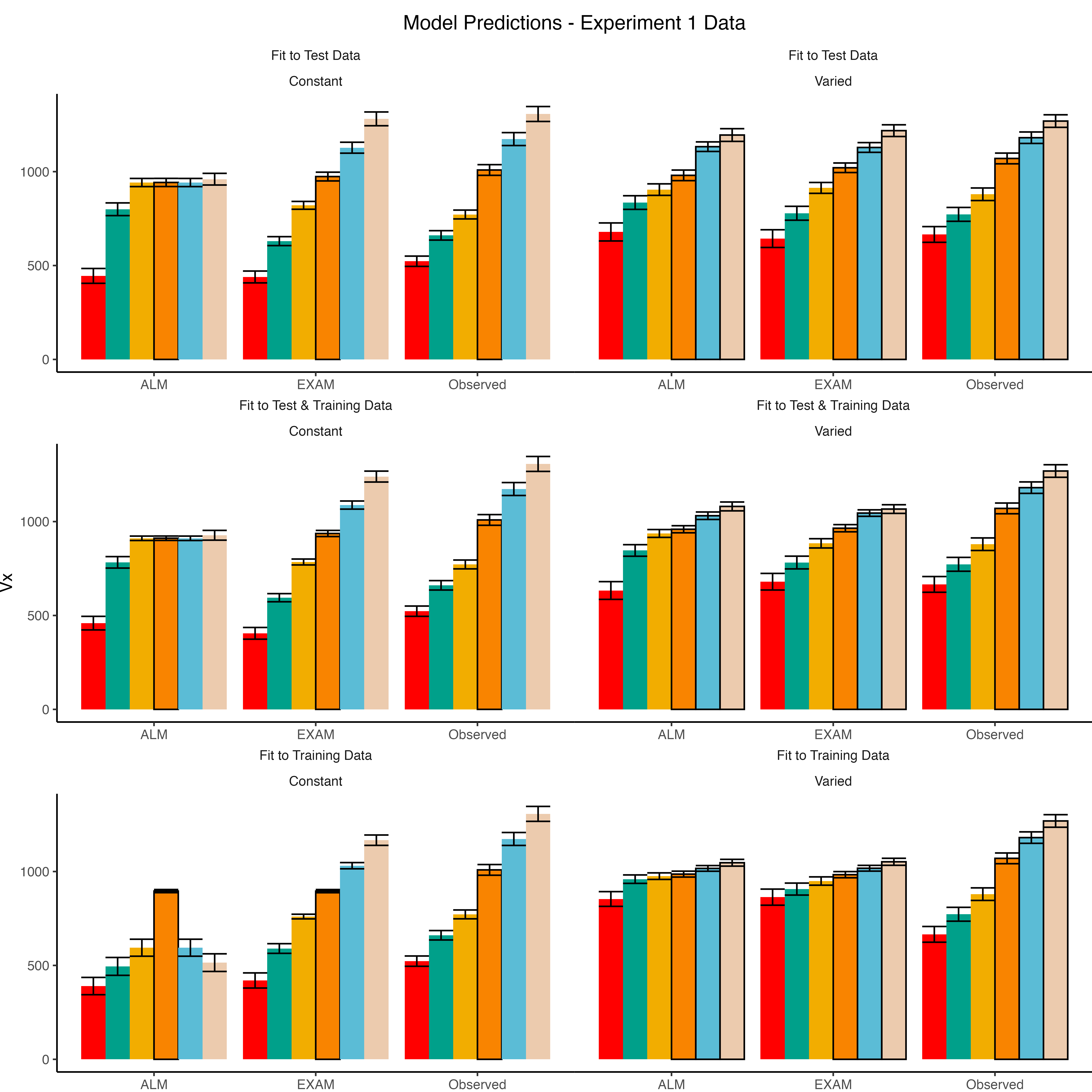
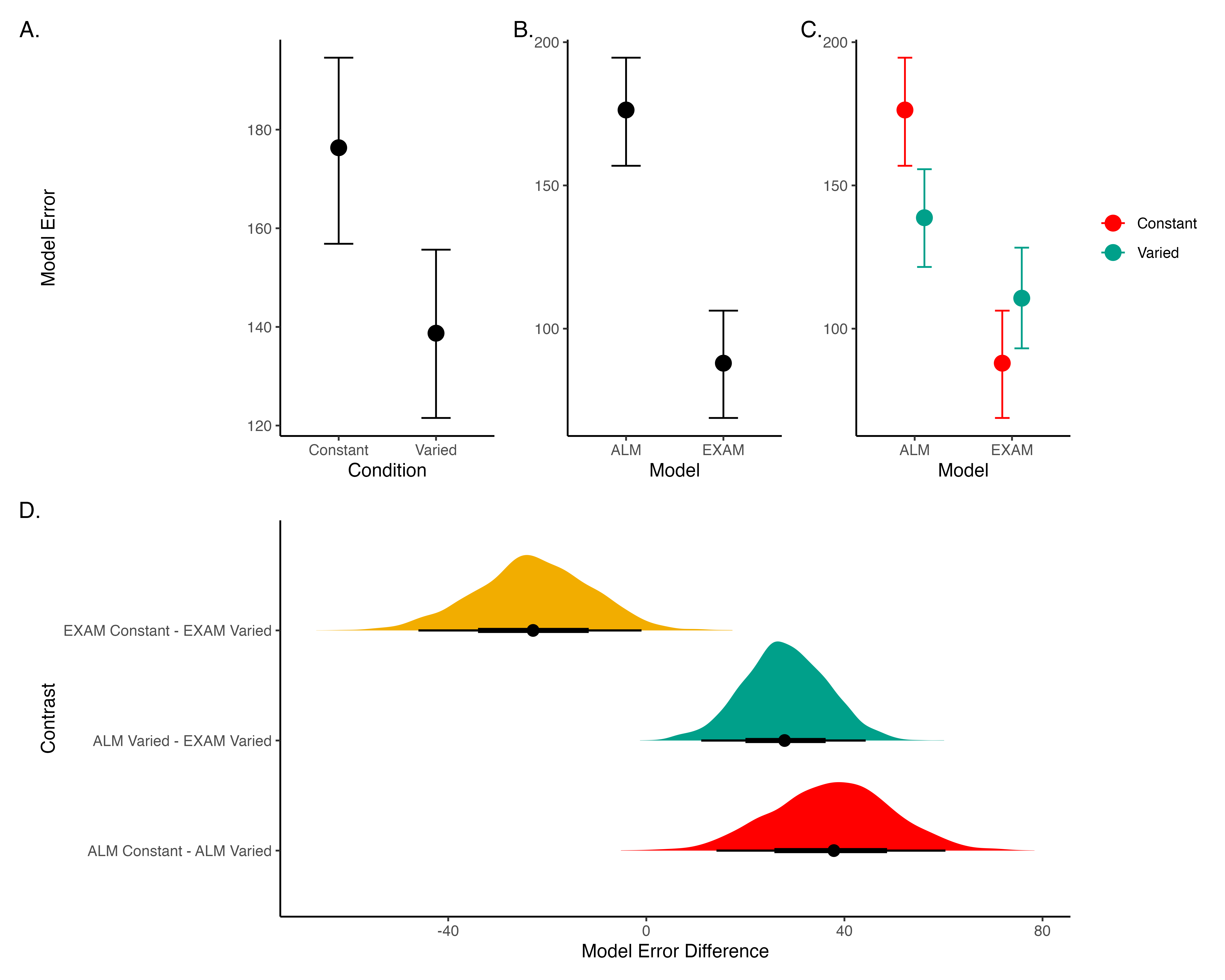
To quantitatively assess the differences in performance between models, we fit a Bayesian regression model predicting the errors of the posterior predictions of each model as a function of the Model (ALM vs. EXAM) and training condition (Constant vs. Varied).
Model errors were significantly lower for EXAM (\(\beta\) = -37.54, 95% CrI [-60.4, -14.17], pd = 99.85%) than ALM. There was also a significant interaction between Model and Condition (\(\beta\) = 60.42, 95% CrI [36.17, 83.85], pd = 100%), indicating that the advantage of EXAM over ALM was significantly greater for the constant group. To assess whether EXAM predicts performance significantly better for Constant than for Varied subjects, we calculated the difference in model error between the Constant and Varied conditions specifically for EXAM. The results indicated that the model error for EXAM was significantly lower in the Constant condition compared to the Varied condition, with a mean difference of -22.88 (95% CrI [-46.02, -0.97], pd = 0.98).
| E2 | E3 | |||||||
|---|---|---|---|---|---|---|---|---|
| Task Stage | ALM | EXAM | ALM | EXAM | ||||
| Constant | Varied | Constant | Varied | Constant | Varied | Constant | Varied | |
| Fit to Test Data | ||||||||
| Test | 239.7 | 129.8 | 99.7 | 88.2 | 170.1 | 106.1 | 92.3 | 72.8 |
| Train | 53.1 | 527.1 | 108.1 | 169.3 | 70.9 | 543.5 | 157.8 | 212.7 |
| Fit to Test & Training Data | ||||||||
| Test | 266.0 | 208.2 | 125.1 | 126.4 | 197.7 | 189.5 | 130.0 | 128.5 |
| Train | 40.0 | 35.4 | 30.4 | 23.6 | 49.1 | 85.6 | 49.2 | 78.4 |
| Fit to Training Data | ||||||||
| Test | 357.4 | 295.9 | 305.1 | 234.5 | 415.0 | 298.8 | 295.5 | 243.7 |
| Train | 42.5 | 23.0 | 43.2 | 22.6 | 51.4 | 63.8 | 51.8 | 65.3 |
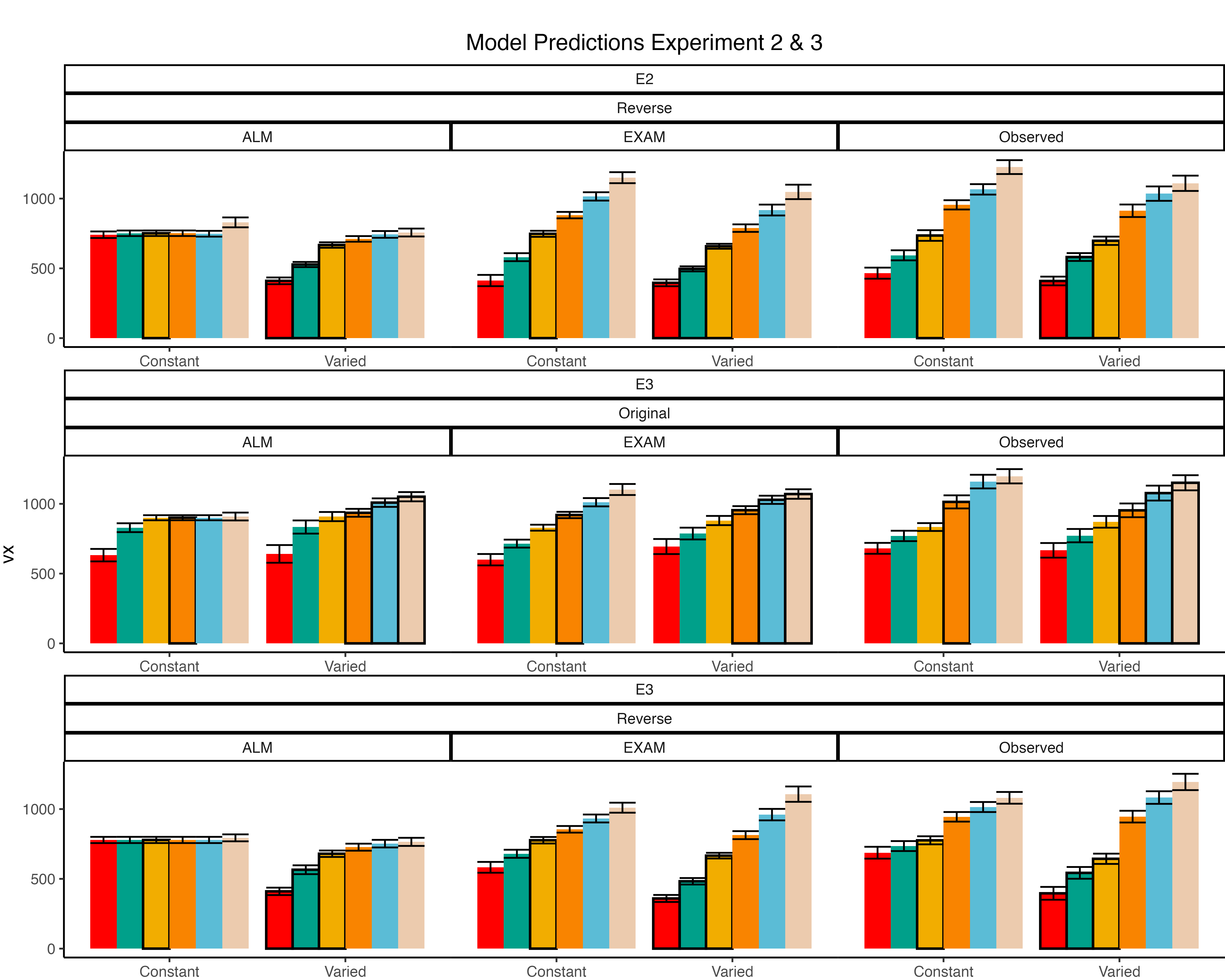
| Experiment | Term | Estimate | Credible Interval | pd | |
|---|---|---|---|---|---|
| 95% CrI Lower | 95% CrI Upper | ||||
| Experiment 1 | |||||
| Exp 1 | Intercept | 176.3 | 156.9 | 194.6 | 1.00 |
| Exp 1 | ModelEXAM | −88.4 | −104.5 | −71.8 | 1.00 |
| Exp 1 | conditVaried | −37.5 | −60.4 | −14.2 | 1.00 |
| Exp 1 | ModelEXAM:conditVaried | 60.4 | 36.2 | 83.8 | 1.00 |
| Experiment 2 | |||||
| Exp 2 | Intercept | 245.9 | 226.2 | 264.5 | 1.00 |
| Exp 2 | ModelEXAM | −137.7 | −160.2 | −115.5 | 1.00 |
| Exp 2 | conditVaried | −86.4 | −113.5 | −59.3 | 1.00 |
| Exp 2 | ModelEXAM:conditVaried | 56.9 | 25.3 | 88.0 | 1.00 |
| Experiment 3 | |||||
| Exp 3 | Intercept | 164.8 | 140.1 | 189.4 | 1.00 |
| Exp 3 | ModelEXAM | −65.7 | −86.0 | −46.0 | 1.00 |
| Exp 3 | conditVaried | −40.6 | −75.9 | −3.0 | 0.98 |
| Exp 3 | bandOrderReverse | 25.5 | −9.3 | 58.7 | 0.93 |
| Exp 3 | ModelEXAM:conditVaried | 41.9 | 11.2 | 72.5 | 0.99 |
| Exp 3 | ModelEXAM:bandOrderReverse | −7.3 | −34.5 | 21.1 | 0.70 |
| Exp 3 | conditVaried:bandOrderReverse | 30.8 | −19.6 | 83.6 | 0.88 |
| Exp 3 | ModelEXAM:conditVaried:bandOrderReverse | −60.6 | −101.8 | −18.7 | 1.00 |
Model Fits to Experiment 2 and 3. Data from Experiments 2 and 3 were fit to ALM and EXAM in the same manner as Experiment 1. For brevity, we only plot and discuss the results of the “fit to training and testing data” models - results from the other fitting methods can be found in the appendix. The model fitting results for Experiments 2 and 3 closely mirrored those observed in Experiment 1. The Bayesian regression models predicting model error as a function of Model (ALM vs. EXAM), Condition (Constant vs. Varied), and their interaction (see Table 18) revealed a consistent main effect of Model across all three experiments. The negative coefficients for the ModelEXAM term (Exp 2: \(\beta\) = -86.39, 95% CrI -113.52, -59.31, pd = 100%; Exp 3: \(\beta\) = -40.61, 95% CrI -75.9, -3.02, pd = 98.17%) indicate that EXAM outperformed ALM in both experiments. Furthermore, the interaction between Model and Condition was significant in both Experiment 2 (\(\beta\) = 56.87, 95% CrI 25.26, 88.04, pd = 99.98%) and Experiment 3 (\(\beta\) = 41.9, 95% CrI 11.2, 72.54, pd = 99.35%), suggesting that the superiority of EXAM over ALM was more pronounced for the Constant group compared to the Varied group, as was the case in Experiment 1. Recall that Experiment 3 included participants in both the original and reverse order conditions - and that this manipulation interacted with the effect of training condition. We thus also controlled for band order in our Bayesian Regression assessing the relative performance of EXAM and ALM in Experiment 3. There was a significant three way interaction between Model, Training Condition, and Band Order (\(\beta\) = -60.6, 95% CrI -101.8, -18.66, pd = 99.83%), indicating that the relative advantage of EXAM over ALM was only more pronounced in the original order condition, and not the reverse order condition (see Figure 33).
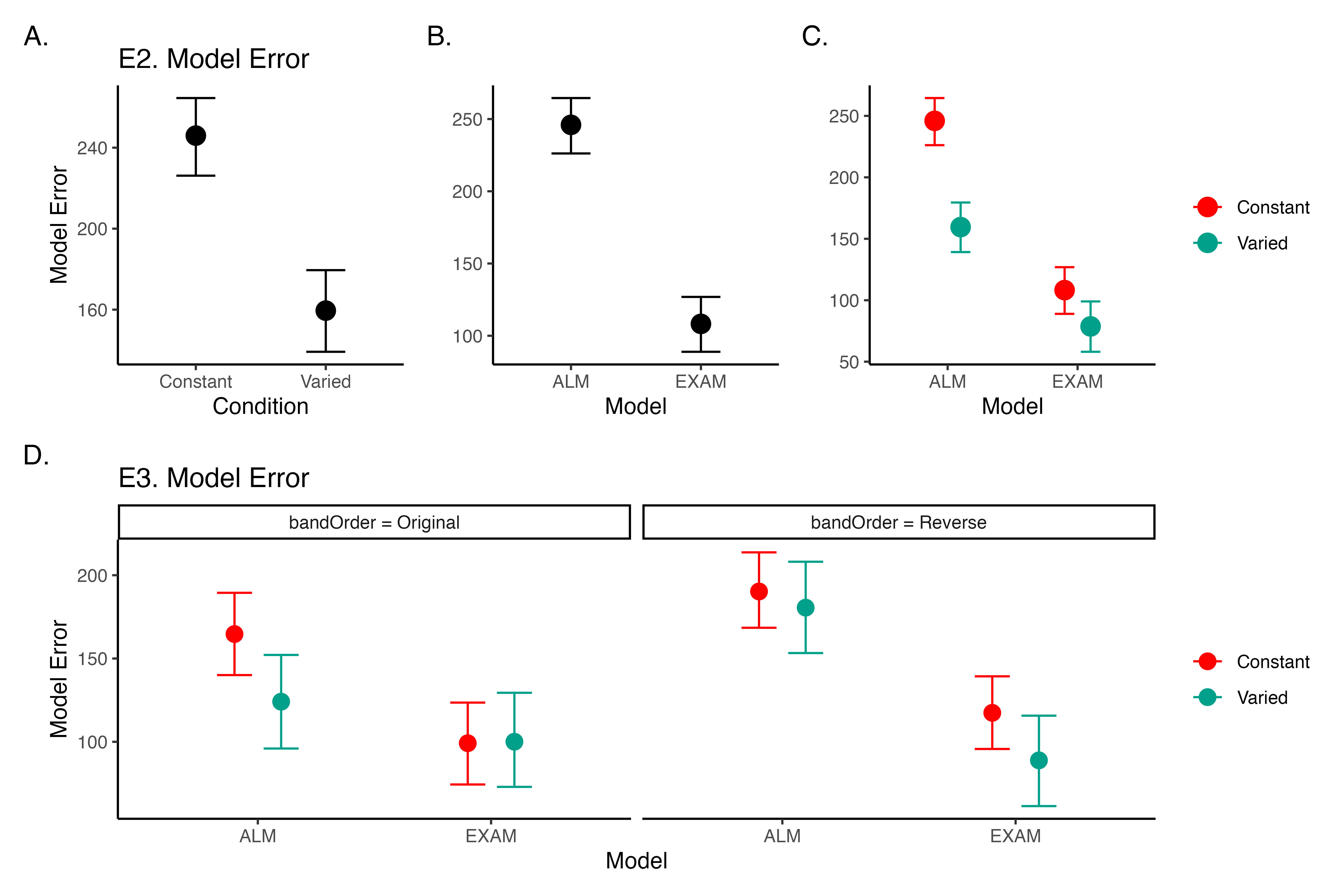
Computational Model Summary. Across all three experiments, the model fits consistently favored the Extrapolation-Association Model (EXAM) over the Associative Learning Model (ALM). This preference for EXAM was particularly pronounced for participants in the constant training conditions (note the positive coefficients on ModelEXAM:conditVaried interaction terms Table 18). This pattern is clearly illustrated in Figure 34, which plots the difference in model errors between ALM and EXAM for each individual participant. Both varied and constant conditions have a greater proportion of subjects better fit by EXAM (positive error differences), with the magnitude of EXAM’s advantage visibly larger for the constant group.
The superior performance of EXAM, especially for the constant training groups, may initially seem counterintuitive. One might assume that exposure to multiple, varied examples would be necessary to extract an abstract rule. However, EXAM is not a conventional rule-based model; it does not require the explicit abstraction of a rule. Instead, rule-based responses emerge during the retrieval process. The constant groups’ formation of a single, accurate input-output association, combined with the usefulness of the zero point, seem to have been sufficient for EXAM to capture their performance. A potential concern is that the assumption of participants utilizing the zero point essentially transforms the extrapolation problem into an interpolation problem. However, this concern is mitigated by the consistency of the results across both the original and reversed order conditions (the testing extrapolation bands fall in between the constant training band and the 0 point in experiment 1, but not in experiment 2).
The fits to the individual participants also reveal a number of interesting cases where the models struggle to capture the data (Figure 35). For example participant 68 exhibits a strong non-monotonicity in the highest velocity band, a pattern which ALM can mimic, but which EXAM cannot capture, given that it enforces a simple linear relationship between target velocity and response. Participant 70 (lower right corner of Figure 35) had a roughly parabolic response pattern in their observed data, a pattern which neither model can properly reproduce, but which causes EXAM to perform particularly poorly.
Modeling Limitations. The present work compared models based on their ability to predict the observed data, without employing conventional model fit indices such as the Akaike Information Criterion (AIC) or the Bayesian Information Criterion (BIC). These indices, which penalize models based on their number of free parameters, would have been of limited utility in the current case, as both ALM and EXAM have two free parameters. However, despite having the same number of free parameters, EXAM could still be considered the more complex model, as it incorporates all the components of ALM plus an additional mechanism for rule-based responding. A more comprehensive model comparison approach might involve performing cross-validation with a held-out subset of the data (Mezzadri et al., 2022) or penalizing models based on the range of patterns they can produce (Dome & Wills, 2023), under the assumption that more constrained models are more impressive when they do adequately fit a given pattern of results.
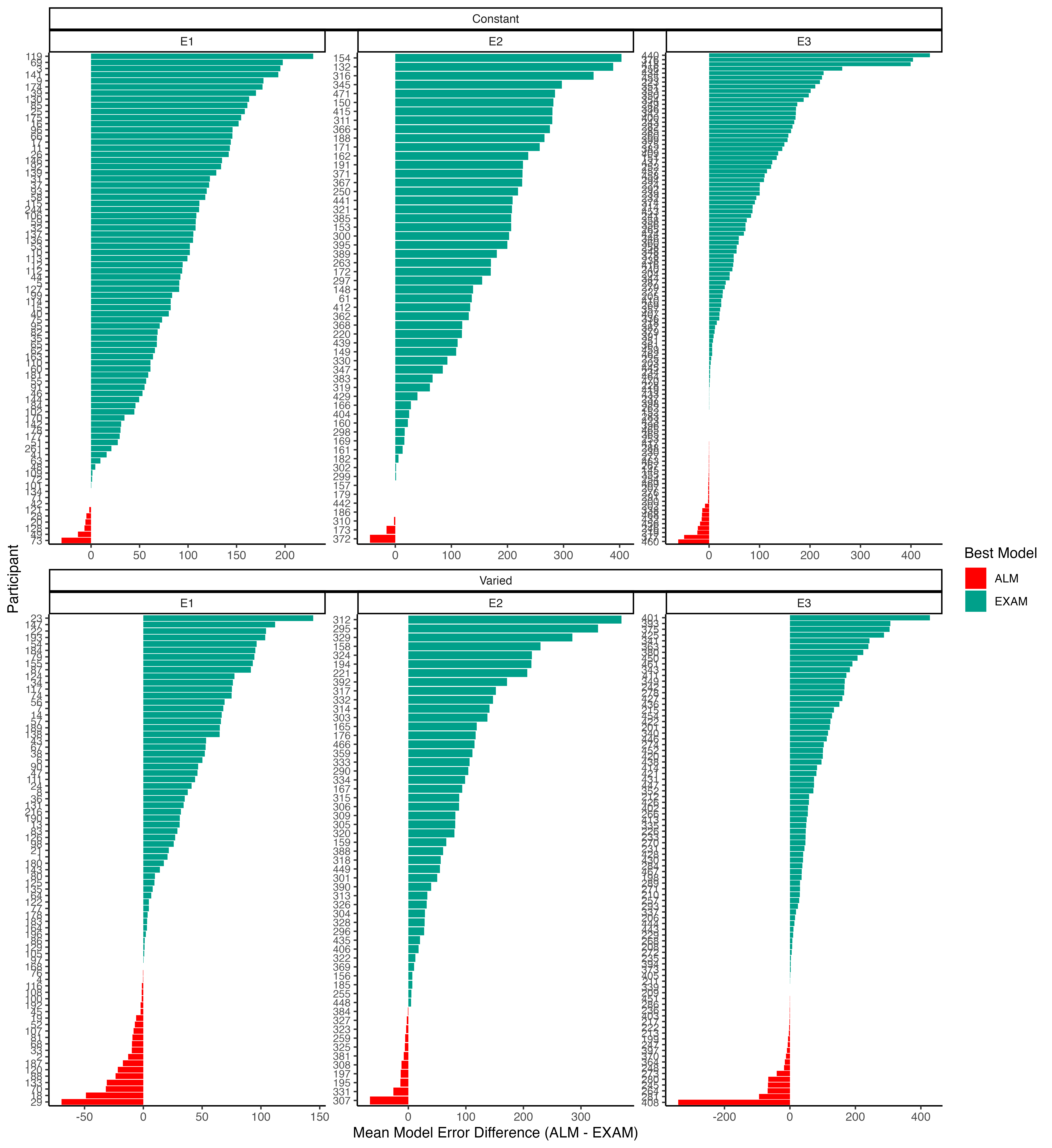

Project 2 Discussion
Across three experiments, we investigated the impact of training variability on learning and extrapolation in a visuomotor function learning task.
In Experiment 1, participants in the varied training condition, who experienced a wider range of velocity bands during training, showed lower accuracy at the end of training compared to those in the constant training condition. Crucially, during the testing phase, the varied group exhibited significantly larger deviations from the target velocity bands, particularly for the extrapolation bands that were not encountered during training. The varied group also showed less discrimination between velocity bands, as evidenced by shallower slopes when predicting response velocity from target velocity band.
Experiment 2 extended these findings by reversing the order of the training and testing bands. Similar to Experiment 1, the varied group demonstrated poorer performance during both training and testing phases. However, unlike Experiment 1, the varied group did not show a significant difference in discrimination between bands compared to the constant group.
In Experiment 3, we provided only ordinal feedback during training, in contrast to the continuous feedback provided in the previous experiments. Participants were assigned to both an order condition (original or reverse) and a training condition (constant or varied). The varied condition showed larger deviations at the end of training, consistent with the previous experiments. Interestingly, there was a significant interaction between training condition and band order, with the varied condition showing greater accuracy in the reverse order condition. During testing, the varied group once again exhibited larger deviations, particularly for the extrapolation bands. The reverse order conditions showed smaller deviations compared to the original order conditions. Discrimination between velocity bands was poorer for the varied group in the original order condition, but not in the reverse order condition.
All three of our experiments yielded evidence that varied training conditions produced less learning by the end of training, a pattern consistent with much of the previous research on the influence of training variability (Catalano & Kleiner, 1984; Soderstrom & Bjork, 2015; Wrisberg et al., 1987). The sole exception to this pattern was the reverse order condition in Experiment 3, where the varied group was not significantly worse than the constant group. Neither the varied condition trained with the same reverse-order items in Experiment 2, nor the original-order varied condition trained with ordinal feedback in Experiment 3 were able to match the performance of their complementary constant groups by the end of training, suggesting that the relative success of the ordinal-reverse ordered varied group cannot be attributed to item or feedback effects alone.
Our findings also diverge from the two previous studies that cleanly manipulated the variability of training items in a function learning task (DeLosh et al., 1997; van Dam & Ernst, 2015), although the varied training condition of van Dam & Ernst (2015) also exhibited less learning, neither of these previous studies observed any difference between training conditions in extrapolation to novel items. Like DeLosh et al. (1997), our participants exhibited above chance extrapolation/discrimination of novel items, however they observed no difference between any of their three training conditions. A noteworthy difference between our studies is that DeLosh et al. (1997) trained participants with either 8, 20, or 50 unique items (all receiving the same total number of training trials). These larger sets of unique items, combined with the fact that participants achieved near ceiling level performance by the end of training, may have made it more difficult to observe any between-group differences of training variation in their study. van Dam & Ernst (2015) ’s variability manipulation was more similar to our own, as they trained participants with either 2 or 5 unique items. However, although the mapping between their input stimuli and motor responses was technically linear, the input dimension was more complex than our own, as it was defined by the degree of “spikiness” of the input shape. This entirely arbitrary mapping also would have precluded any sensible “0” point, which may partially explain why neither of their training conditions were able to extrapolate linearly in the manner observed in the current study or in DeLosh et al. (1997).
To explain our results, we turned to the well established EXAM and ALM models. The disproportionate success of EXAM in capturing the performance of participants under the constant training condition suggests that rule-based extrapolation can emerge even from a limited set of training examples. This success hinges on the assumption that participants are able to leverage prior knowledge of the zero-point reference (Brown & Lacroix, 2017; Kwantes & Neal, 2006). The zero-point reference, combined with accurate learning of the single trained velocity band enabled EXAM to capture the extrapolation patterns of the constant participants. However, it’s important to acknowledge that the ALM model provided a better fit for a subset of participants in each of our three experiment, highlighting the presence of substantial individual differences in generalization patterns.
This finding illustrates the importance of considering task structure when evaluating the effects of training variability on generalization and extrapolation. Some tasks, like the one in this study, may permit the use of zero-point knowledge or other prior information, while others may not. For example, a zero point may be less relevant in visuomotor tasks with complex rotations (Roller et al., 2001; van Dam & Ernst, 2015), or in complex sports techniques (North et al., 2019). Future research should systematically investigate how different task structures interact with training variability to influence learning outcomes and generalization abilities, taking into account factors such as the availability of prior knowledge, the complexity of the task, and the specific learning mechanisms involved. This approach could help reconcile seemingly contradictory findings in the literature and provide more nuanced guidelines for designing effective training protocols across various domains.
Limitations
While the present study provides valuable insights into the influence of training variability on visuomotor function learning and extrapolation, there are several limitations that should be flagged. First, although the constant training group never had experience from a velocity band closer to the extrapolation bands than the varied group, they always had three times more trials with the nearest velocity band. Such a difference may be an unavoidable consequence of a varied vs. constant design which matches the total number of training trials between the two groups. However, in order to more carefully tease apart the influence of variability from the influence of frequency/repetition effects, future research could explore alternative designs that maintain the variability manipulation while equating the amount of training on the nearest examples across conditions, such as by increasing the total number of trials for the varied group. Another limitation is that the testing stage did not include any interpolation items, i.e. the participants were tested only from the training bands they experienced during training, or from extrapolation bands. The absence of interpolation testing makes it more difficult to distinguish between the effects of training variability on extrapolation specifically, as opposed to generalization more broadly. Of course, the nature of the constant training condition makes interpolation testing impossible to implement, however future studies might compare training regimes that each include at least 2 distinct items, but still differ in the total amount of variability experienced, which would then allow groups to be compared in terms of both interpolation and extrapolation testing. Finally, the task employed in the present study consisted of only a linear, positive function. Previous work in human function learning has repeatedly shown that such functions are among the easiest to learn, but that humans are nonetheless capable of learning negative, non-linear, or discontinuous functions (Busemeyer et al., 1997; DeLosh et al., 1997; Kalish, 2013; McDaniel et al., 2009). It thus remains an open question as to whether the influence of training variability might interact with various components of the to-be-learned function.
General Discussion
To facilitate ease of comparison between the two projects and their respective tasks, we’ll now refer to project 1 as Hit The Target (HTT) and project 2 as Hit The Wall (HTW).
Empirical and Modeling Summary
Across both projects, we investigated the influence of training variability on learning and generalization in computerized visuomotor skill learning, and function learning tasks. In project 1 (HTT), experiments 1 and 2 demonstrated that varied training led to superior testing performance compared to constant training. In Experiment 1, the varied group even outperformed the constant group even when testing from the constant groups trained position. In contrast, Project 2 (HTW) found the opposite pattern - the varied training groups exhibited poorer performance than the constant groups, both in terms of training accuracy, accuracy in extrapolation testing, and, in a subset of the experiments, the varied group showed a diminished ability to discriminate between bands. This detrimental effect of variability was observed across three experiments, with the exception of the reverse order condition in Experiment 3, where the varied group was able to match the constant group’s performance.
Both projects also included computational modeling componenents. In Project 1, the IGAS model was introduced as a means of addressing the lack of control for similarity between training and testing conditions common to previous work in the “benefits of variability” literature. The IGAS model provides a theoretically motivated method of quantifying the similarity between training experience and testing conditions. The resulting similarity metric (i.e. our 1c-similarity) is shown to be a significant predictor of testing performance on its own, and when added as a covariate to the statistical model used to compare the constant and varied training groups. We then showed the group-level effect of training variability on testing performance can be accounted for with the additional assumption that training variability influences the generalization gradient. The contribution of the IGAS model was thus twofold: 1) providing a theoretically justifiable method of quantifying/controlling for similarity between training and testing, and 2) demonstrating the viability of a flexible-similarity based generalization account for the empirically observed benefit of variability in our task. Although similar approaches have been employed in other domains, both contributions are novel additions to the large body of research assessing the effect of constant vs. varied training manipulations in visuomotor skill tasks.
Although theoretically motivated, the IGAS model of Project 1 is best categorized as a descriptive measurement-model. Sufficient to account for group differences, but lacking the machinery necessary to provide a full process-level account of how the empirical quantities of interest are generated. In contrast, Project 2 (HTW) implemented a more robust computational modeling approach, implementing and comparing full process models (ALM & EXAM), capable of generating predictions for both the learning and testing stages of the experiment. ALM and EXAM have been used as models of function learning, cue judgement, and forecasting behavior in numerous studies over the past 25 years (Brown & Lacroix, 2017; DeLosh et al., 1997; Kane & Broomell, 2020; H. Kelley & Busemeyer, 2008; Kwantes et al., 2012; McDaniel et al., 2009; Von Helversen & Rieskamp, 2010). The present work presents the first application of these models to the study of training variability in a visuomotor function learning task. We fit both models to individual participant data, using a form of simulation-based Bayesian parameter estimation that allowed us to generate and compare the full posterior predictive distributions of each model. EXAM provided the best overall account of the testing data, and the advantage of EXAM over ALM was significantly greater for the constant group. Notably, EXAM captured the constant groups’ ability to extrapolate linearly to novel velocity bands, despite receiving training from only a single input-output pair. This finding suggests that EXAM’s linear extrapolation mechanism, combined with the assumption of prior knowledge about the origin point (0, 0), was sufficient to account for the constant groups’ accurate extrapolation performance. Such findings may offer a preliminary suggestion that experience with a more variable set of training examples may be detrimental to performance in simple extrapolation tasks.
Differences between the two Projects
The HTT and HTW tasks differ across numerous dimensions that may be relevant to the opposing patterns observed in the two projects (see Table 19 for a detailed comparison of the two tasks).
In HTT, the salient perceptual elements of the task (i.e. the launching box, target and barrier) are subject to variation (i.e. different distances between the launching box and target), and the spatial layout of these perceptually variable elements are intrinsically linked to the task objective of striking the target. Conversely, the perceptual task elements in HTW are invariant across trials, and the task objective is specified by the target velocity value specified as a numeral at the top of the screen. If the benefits of training variation do arise from the formation and flexible retrieval of distinct memory traces, then the lack of perceptual salience between training instances in the HTW task may have limited any potential benefits of variability. Future work could investigate this possibility further employing a modified version of the HTW task wherein the correct velocity value is indicated by some perceptual feature of the task (e.g., the color of the wall, or size of the ball), rather than displaying the target velocity numerically.
The HTT and HTW tasks also differed in terms of general task complexity. The HTT task was designed to mimic projectile launching tasks commonly employed in visuomotor learning studies, and the parabolic trajectories necessary to strike the target in HTT were sensitive to both the x and y dimensions of the projectiles velocity (and to a lesser extent, the position within the launching box at which the ball was released). Conversely the HTW task was influenced to a greater extent by the tasks commonly utilized in the function learning literature, wherein the correct output responses are determined by a single input dimension. In HTW, the relationship between feedback and optimal behavioral adjustment is also almost perfectly smooth, if participants produce a throw that is 100 units too hard, they’ll be told that they were 100 units away from the target band. Whereas in HTT, the presence of the barrier in introduces irregularities in the task space. Even throws close to the solution space might result in failure, creating a less predictable learning environment.
| Dimension | HTT (Project 1) | HTW (Project 2) |
|---|---|---|
| Task Description | Projectile launching to hit a target | Projectile launching to hit wall at a specific velocity |
| Task Complexity | More complex parabolic trajectory, both x and y velocities relevant to outcome | Simpler 1D mapping of force to outcome. Only x velocity is relevant. |
| Task Space | More complex: xy velocity combinations closer to the solution space may still result in worse feedback due to striking the barrier. | Simpler: smooth, linear mapping between velocity and feedback. |
| Perceptual salience of Varied Conditions | Varied conditions (# of throwing distances) are perceptually distinct, i.e. salient differences in distance between launching box and target. | Varied conditions (# of velocity bands) are less salient - only difference is the numeral displayed on screen. |
| Testing Feedback | Testing always included feedback | Primary testing stage had no feedback. |
| Potential for Learning during Testing | Limited potential for learning during testing due to feedback. | Some potential for learning during no-feedback testing by observing ball trajectory. |
| Training Experience | Varied group gets half as much experience on any one position as the constant group. | Varied group gets 1/3 as much experience on any one velocity band as the constant group. |
| Testing Structure | Random interleaving of trained/transfer testing distances. | Blocked structure, separately testing trained vs extrapolation testing bands. |
It is important to note that while both projects utilize computational models, direct comparisons are complicated by the distinct purposes and structures of the models used in each project. The IGAS model of Project 1 serves as a descriptive measurement model, capturing the similarity between training throws and testing conditions. In contrast, the ALM and EXAM models of Project 2 are full process models, capable of generating exact predictions for both learning and testing stages. The difference is also reflected in the interpretion of the generalization parameter (\(c\)) across the models of the two projects. In IGAS, \(c\) moderates the similarity between executed throws and subsequent testing solutions, while in ALM and EXAM, \(c\) governs the extent to which the perceived stimuli activate the input layer nodes. Despite these differences, insights from ALM/EXAM, particularly the role of zero-point knowledge, may offer potential explanations for the contrasting empirical results. Particularly, EXAM’s reliance on zero-point knowledge in the simpler HTW task may explain why constant training was more effective in Project 2, while the lack of a clear zero-point reference in the more complex HTT task of Project 1 may have increased the value of varied training. This suggests that the benefits of variability depend critically on how task structure interacts with prior knowledge and the learner’s capacity to leverage such knowledge for generalization.
Future work could explore extending ALM and EXAM, which have traditionally been applied to one-dimensional function learning tasks, to more complex motor tasks such as HTT. The neural network structure of ALM could be adapted to handle 2D input by utilizing a 2D grid of input nodes, allowing the model to learn mappings between 2D throwing velocities and desired outcomes. This would allow the model to process the more complex spatial information inherent in tasks like HTT. Furthermore, the output layers of ALM/EXAM could be expanded to express more complex motor outputs in addition to velocity, such as the locations of grabbing and releasing the projectile or other parameters defining the unique trajectories produced. In addition to allowing the models to be applied to more complex tasks, these modifications could enable researchers to investigate how perceptual similarity (i.e., the similarity of stimuli) and motoric similarity (i.e., the similarity of behavioral actions) may separately and jointly influence learning and generalization.
Conclusion
In summary, this dissertation provides a comprehensive examination of the effects of training variability on learning and generalization in visuomotor and function learning tasks. The contrasting results obtained from the Hit The Target (HTT) and Hit The Wall (HTW) tasks underscore the complexity inherent to the longstanding pedagogical and scientific goal of identifying training manipulations that consistently benefit learning and generalization. Moreover, through the development and application of computational models, we provide novel theoretical accounts for both the beneficial and detrimental effects of training variability observed in our experiments. These findings highlight the importance of considering task characteristics when designing experiments intended to assess the influence of training interventions, and demonstrate the value of combining empirical and computational modeling approaches to uncover the cognitive mechanisms that support learning and generalization. Future research should continue to investigate the complex interplay between task demands, training manipulations, and individual differences, with the goal of optimizing educational and training outcomes across a wide range of domains.
Appendix
Apppendix available at https://tegorman13.github.io/Dissertation/Sections/Appendix/Full_Appendix.html
References
Aha, D. W., & Goldstone, R. L. (1992). Concept Learning and Flexible Weighting. In Proceedings of the Fourteenth Annual Conference of the Cognitive Science Society, 534–539.
Bengtsson, H. (2021). A Unifying Framework for Parallel and Distributed Processing in R using Futures. The R Journal, 13(2), 208. https://doi.org/10.32614/RJ-2021-048
Berniker, M., Mirzaei, H., & Kording, K. P. (2014). The effects of training breadth on motor generalization. Journal of Neurophysiology, 112(11), 2791–2798. https://doi.org/10.1152/jn.00615.2013
Bjork, E. L., & Bjork, R. A. (2011). Making things hard on yourself, but in a good way: Creating desirable difficulties to enhance learning. Psychology and the Real World: Essays Illustrating Fundamental Contributions to Society, 2, 59–68.
Bott, L., & Heit, E. (2004). Nonmonotonic Extrapolation in Function Learning. Journal of Experimental Psychology: Learning, Memory, and Cognition, 30(1), 38–50. https://doi.org/10.1037/0278-7393.30.1.38
Bowman, C. R., & Zeithamova, D. (2020). Training set coherence and set size effects on concept generalization and recognition. Journal of Experimental Psychology. Learning, Memory, and Cognition, 46(8), 1442–1464. https://doi.org/10.1037/xlm0000824
Braithwaite, D. W., & Goldstone, R. L. (2015). Effects of Variation and Prior Knowledge on Abstract Concept Learning. Cognition and Instruction, 33(3), 226–256. https://doi.org/10.1080/07370008.2015.1067215
Braun, D. A., Aertsen, A., Wolpert, D. M., & Mehring, C. (2009). Motor Task Variation Induces Structural Learning. Current Biology, 19(4), 352–357. https://doi.org/10.1016/j.cub.2009.01.036
Brehmer, B. (1974). Hypotheses about relations between scaled variables in the learning of probabilistic inference tasks. Organizational Behavior and Human Performance, 11(1), 1–27. https://doi.org/10.1016/0030-5073(74)90002-6
Brekelmans, G., Lavan, N., Saito, H., Clayards, M., & Wonnacott, E. (2022). Does high variability training improve the learning of non-native phoneme contrasts over low variability training? A replication. Journal of Memory and Language, 126, 104352. https://doi.org/10.1016/j.jml.2022.104352
Breslin, G., Hodges, N. J., Steenson, A., & Williams, A. M. (2012). Constant or variable practice: Recreating the especial skill effect. Acta Psychologica, 140(2), 154–157. https://doi.org/10.1016/j.actpsy.2012.04.002
Briscoe, E., & Feldman, J. (2011). Conceptual complexity and the bias/variance tradeoff. Cognition, 118(1), 2–16. https://doi.org/10.1016/j.cognition.2010.10.004
Brown, M. A., & Lacroix, G. (2017). Underestimation in linear function learning: Anchoring to zero or x-y similarity? Canadian Journal of Experimental Psychology/Revue Canadienne de Psychologie Expérimentale, 71(4), 274–282. https://doi.org/10.1037/cep0000129
Brunstein, A., & Gonzalez, C. (2011). Preparing for novelty with diverse training. Applied Cognitive Psychology, 25(5), 682–691. https://doi.org/10.1002/acp.1739
Bürkner, P.-C. (2017). Brms: An R Package for Bayesian Multilevel Models Using Stan. Journal of Statistical Software, 80, 1–28. https://doi.org/10.18637/jss.v080.i01
Burton, A. M., Kramer, R. S. S., Ritchie, K. L., & Jenkins, R. (2016). Identity From Variation: Representations of Faces Derived From Multiple Instances. Cognitive Science, 40(1), 202–223. https://doi.org/10.1111/cogs.12231
Busemeyer, J. R., Byun, E., DeLosh, E. L., & McDaniel, M. A. (1997). Learning Functional Relations Based on Experience with Input-output Pairs by Humans and Artificial Neural Networks. In Knowledge Concepts and Categories (pp. 405–437). Psychology Press.
Carroll, J. D. (1963). Functional Learning: The Learning of Continuous Functional Mappings Relating Stimulus and Response Continua. ETS Research Bulletin Series, 1963(2), i–144. https://doi.org/10.1002/j.2333-8504.1963.tb00958.x
Catalano, J. F., & Kleiner, B. M. (1984). Distant Transfer in Coincident Timing as a Function of Variability of Practice. Perceptual and Motor Skills, 58(3), 851–856. https://doi.org/10.2466/pms.1984.58.3.851
Censor, N., Sagi, D., & Cohen, L. G. (2012). Common mechanisms of human perceptual and motor learning. Nature Reviews Neuroscience, 13(9), 658–664. https://doi.org/10.1038/nrn3315
Chamberlin, C. J., & Magill, R. A. (1992a). A Note on Schema and Exemplar Approaches to Motor Skill Representation in Memory. Journal of Motor Behavior, 24(2), 221–224. https://doi.org/10.1080/00222895.1992.9941617
Chamberlin, C. J., & Magill, R. A. (1992b). The Memory Representation of Motor Skills: A Test of Schema Theory. Journal of Motor Behavior, 24(4), 309–319. https://doi.org/10.1080/00222895.1992.9941627
Chua, L.-K., Dimapilis, M. K., Iwatsuki, T., Abdollahipour, R., Lewthwaite, R., & Wulf, G. (2019). Practice variability promotes an external focus of attention and enhances motor skill learning. Human Movement Science, 64, 307–319. https://doi.org/10.1016/j.humov.2019.02.015
Ciccione, L., & Dehaene, S. (2021). Can humans perform mental regression on a graph? Accuracy and bias in the perception of scatterplots. Cognitive Psychology, 128, 101406. https://doi.org/10.1016/j.cogpsych.2021.101406
Cochrane, A. (2020). TEfits: Nonlinear regression for time-evolving indices. Journal of Open Source Software, 5(52), 2535. https://doi.org/10.21105/joss.02535
Cohen, A. L., Nosofsky, R. M., & Zaki, S. R. (2001). Category variability, exemplar similarity, and perceptual classification. Memory & Cognition, 29(8), 1165–1175. https://doi.org/10.3758/BF03206386
Cohen, R. G., & Rosenbaum, D. A. (2004). Where grasps are made reveals how grasps are planned: Generation and recall of motor plans. Experimental Brain Research, 157(4). https://doi.org/10.1007/s00221-004-1862-9
Cornwall, A. C., Davis, T., Byrne, K. A., & Worthy, D. A. (2022). Effects of categorical and numerical feedback on category learning. Cognition, 225, 105163. https://doi.org/10.1016/j.cognition.2022.105163
Courrieu, P. (2012). Quick approximation of bivariate functions. British Journal of Mathematical and Statistical Psychology, 65(1), 89–121. https://doi.org/10.1111/j.2044-8317.2011.02016.x
Cranmer, K., Brehmer, J., & Louppe, G. (2020). The frontier of simulation-based inference. Proceedings of the National Academy of Sciences, 117(48), 30055–30062. https://doi.org/10.1073/pnas.1912789117
Crump, M. J. C., & Logan, G. D. (2010). Episodic contributions to sequential control: Learning from a typist’s touch. Journal of Experimental Psychology: Human Perception and Performance, 36(3), 662–672. https://doi.org/10.1037/a0018390
Czyż, S. H. (2021). Variability of Practice, Information Processing, and Decision Making—How Much Do We Know? Frontiers in Psychology, 12. https://doi.org/10.3389/fpsyg.2021.639131
de Leeuw, J. R. (2015). jsPsych: A JavaScript library for creating behavioral experiments in a Web browser. Behavior Research Methods, 47(1), 1–12. https://doi.org/10.3758/s13428-014-0458-y
Del Rey, P., Wughalter, E. H., & Whitehurst, M. (1982). The Effects of Contextual Interference on Females With Varied Experience in Open Sport Skills. Research Quarterly for Exercise and Sport, 53(2), 108–115. https://doi.org/10.1080/02701367.1982.10605236
DeLosh, E. L., McDaniel, M. A., & Busemeyer, J. R. (1997). Extrapolation: The Sine Qua Non for Abstraction in Function Learning. Journal of Experimental Psychology: Learning, Memory, and Cognition, 23(4), 19. https://doi.org/10.1037/0278-7393.23.4.968
Dome, L., & Wills, A. (2023). G-distance: On the comparison of model and human heterogeneity [Preprint]. PsyArXiv. https://doi.org/10.31234/osf.io/ygmcj
Doyle, M. E., & Hourihan, K. L. (2016). Metacognitive monitoring during category learning: How success affects future behaviour: Memory. Memory, 24(9), 1197–1207. https://doi.org/10.1080/09658211.2015.1086805
Ennis, D. M., Palen, J. J., & Mullen, K. (1988). A multidimensional stochastic theory of similarity. Journal of Mathematical Psychology, 32(4), 449–465. https://doi.org/10.1016/0022-2496(88)90023-5
Estes, W. K. (1994). Classification and Cognition. Oxford University Press.
Fan, M., Zhang, D., Zhao, S., Xie, Q., Chen, W., Jie, J., Wang, Y., & Zheng, X. (2022). Stimulus diversity increases category-based fear generalization and the effect of intolerance of uncertainty. Behaviour Research and Therapy, 159, 104201. https://doi.org/10.1016/j.brat.2022.104201
Farrell, S., & Lewandowsky, S. (2018). Computational Modeling of Cognition and Behavior: (1st ed.). Cambridge University Press. https://doi.org/10.1017/CBO9781316272503
Faul, F., Erdfelder, E., Buchner, A., & Lang, A.-G. (2009). Statistical power analyses using G*Power 3.1: Tests for correlation and regression analyses. Behavior Research Methods, 41(4), 1149–1160. https://doi.org/10.3758/BRM.41.4.1149
Fulvio, J. M., Green, C. S., & Schrater, P. R. (2014). Task-Specific Response Strategy Selection on the Basis of Recent Training Experience. PLOS Computational Biology, 10(1), e1003425. https://doi.org/10.1371/journal.pcbi.1003425
Gandolfo, F., Mussa-Ivaldi, F. A., & Bizzi, E. (1996). Motor learning by field approximation. Proceedings of the National Academy of Sciences, 93(9), 3843–3846. https://doi.org/10.1073/pnas.93.9.3843
George, N., & Egner, T. (2021). Stimulus variability and task relevance modulate binding-learning. Attention, Perception, & Psychophysics. https://doi.org/10.3758/s13414-021-02338-6
Gershman, S. J., & Cikara, M. (2023). Structure learning principles of stereotype change. Psychonomic Bulletin & Review, 30(4), 1273–1293. https://doi.org/10.3758/s13423-023-02252-y
Ghahramani, Z., Wolpert, D. M., & Jordan, M. I. (1996). Generalization to Local Remappings of the Visuomotor Coordinate Transformation. Journal of Neuroscience, 16(21), 7085–7096. https://doi.org/10.1523/JNEUROSCI.16-21-07085.1996
Gonzalez, C., & Madhavan, P. (2011). Diversity during training enhances detection of novel stimuli. Journal of Cognitive Psychology, 23(3), 342–350. https://doi.org/10.1080/20445911.2011.507187
Goode, M. K., Geraci, L., & Roediger, H. L. (2008). Superiority of variable to repeated practice in transfer on anagram solution. Psychonomic Bulletin & Review, 15(3), 662–666. https://doi.org/10.3758/PBR.15.3.662
Goodwin, J. E., Eckerson, J. M., Grimes, C. R., & Gordon, P. M. (1998). Effect of Different Quantities of Variable Practice on Acquisition, Retention, and Transfer of An Applied Motor Skill. Perceptual and Motor Skills, 87(1), 147–151. https://doi.org/10.2466/pms.1998.87.1.147
Gorman, T. E., & Goldstone, R. L. (2022). An instance-based model account of the benefits of varied practice in visuomotor skill. Cognitive Psychology, 137, 101491. https://doi.org/10.1016/j.cogpsych.2022.101491
Green, D. P., Whitehead, J., & Sugden, D. A. (1995). Practice Variability and Transfer of a Racket Skill. Perceptual and Motor Skills, 81(3_suppl), 1275–1281. https://doi.org/10.2466/pms.1995.81.3f.1275
Guadagnoli, M. A., Holcomb, W. R., & Weber, T. J. (1999). The relationship between contextual interference effects and performer expertise on the learning of a putting task. Journal of Human Movement Studies, 37(1), 19–36.
Guadagnoli, M. A., & Lee, T. D. (2004). Challenge Point: A Framework for Conceptualizing the Effects of Various Practice Conditions in Motor Learning. Journal of Motor Behavior, 36(2), 212–224. https://doi.org/10.3200/JMBR.36.2.212-224
Guo, J.-P., Yang, L.-Y., & Ding, Y. (2014). Effects of example variability and prior knowledge in how students learn to solve equations. European Journal of Psychology of Education, 29(1), 21–42. https://www.jstor.org/stable/43551124
Hacques, G., Dicks, M., Komar, J., & Seifert, L. (2022). Visual control during climbing: Variability in practice fosters a proactive gaze pattern. PLOS ONE, 17(6), e0269794. https://doi.org/10.1371/journal.pone.0269794
Hahn, U., Bailey, T. M., & Elvin, L. B. C. (2005). Effects of category diversity on learning, memory, and generalization. Memory & Cognition, 33(2), 289–302. https://doi.org/10.3758/BF03195318
Hills, T. T., Todd, P. M., & Goldstone, R. L. (2010). The central executive as a search process: Priming exploration and exploitation across domains. Journal of Experimental Psychology: General, 139(4), 590–609. https://doi.org/10.1037/a0020666
Hintzman, D. L. (1984). MINERVA 2: A simulation model of human memory. Behavior Research Methods, Instruments, & Computers, 16(2), 96–101. https://doi.org/10.3758/BF03202365
Hintzman, D. L. (1986). "Schema abstraction" in a multiple-trace memory model. Psychological Review, 93(4), 411.
Homa, D., & Vosburgh, R. (1976). Category breadth and the abstraction of prototypical information. Journal of Experimental Psychology: Human Learning and Memory, 2(3), 322–330. https://doi.org/10.1037/0278-7393.2.3.322
Hommel, B. (1998). Event Files: Evidence for Automatic Integration of Stimulus-Response Episodes. Visual Cognition, 5(1-2), 183–216. https://doi.org/10.1080/713756773
Honig, T., Shoham, A., & Yovel, G. (2022). Perceptual similarity modulates effects of learning from variability on face recognition. Vision Research, 201, 108128. https://doi.org/10.1016/j.visres.2022.108128
Hosch, A.-K., Wirtz, P., & von Helversen, B. (2023). Prior Experience of Variability Influences Generalization of Unspecified Categories. Quarterly Journal of Experimental Psychology (2006), 17470218231210491. https://doi.org/10.1177/17470218231210491
Hsu, A. S., & Griffiths, T. L. (2010). Effects of generative and discriminative learning on use of category variability. 32nd Annual Conference of the Cognitive Science Society, 7.
Hu, M., & Nosofsky, R. M. (2024). High-variability training does not enhance generalization in the prototype-distortion paradigm. Memory & Cognition, 1–16. https://doi.org/10.3758/s13421-023-01516-1
Huet, M., Jacobs, D. M., Camachon, C., Missenard, O., Gray, R., & Montagne, G. (2011). The education of attention as explanation of variability of practice effects: Learning the final approach phase in a flight simulator. Journal of Experimental Psychology: Human Perception and Performance, 37(6), 1841–1854. https://doi.org/10.1037/a0024386
Jamieson, R. K., Johns, B. T., Vokey, J. R., & Jones, M. N. (2022). Instance theory as a domain-general framework for cognitive psychology. Nature Reviews Psychology, 1(3), 174–183. https://doi.org/10.1038/s44159-022-00025-3
Jones, S. D., & Brandt, S. (2020). Density and Distinctiveness in Early Word Learning: Evidence From Neural Network Simulations. Cognitive Science, 44(1), e12812. https://doi.org/10.1111/cogs.12812
Kalish, M. L. (2013). Learning and extrapolating a periodic function. Memory & Cognition, 41(6), 886–896. https://doi.org/10.3758/s13421-013-0306-9
Kalish, M. L., Lewandowsky, S., & Kruschke, J. K. (2004). Population of Linear Experts: Knowledge Partitioning and Function Learning. Psychological Review, 111(4), 1072–1099. https://doi.org/10.1037/0033-295X.111.4.1072
Kane, P. B., & Broomell, S. B. (2020). Applications of the bias–variance decomposition to human forecasting. Journal of Mathematical Psychology, 98, 102417. https://doi.org/10.1016/j.jmp.2020.102417
Kangasrääsiö, A., Jokinen, J. P. P., Oulasvirta, A., Howes, A., & Kaski, S. (2019). Parameter Inference for Computational Cognitive Models with Approximate Bayesian Computation. Cognitive Science, 43(6), e12738. https://doi.org/10.1111/cogs.12738
Kassambara, A. (2021). Rstatix: Pipe-Friendly Framework for Basic Statistical Tests.
Kelley, H., & Busemeyer, J. (2008). A comparison of models for learning how to dynamically integrate multiple cues in order to forecast continuous criteria. Journal of Mathematical Psychology, 52(4), 218–240. https://doi.org/10.1016/j.jmp.2008.01.009
Kelley, T. A., & Yantis, S. (2009). Learning to attend: Effects of practice on information selection. Journal of Vision, 9(7), 16. https://doi.org/10.1167/9.7.16
Kerr, R., & Booth, B. (1978). Specific and varied practice of motor skill. Perceptual and Motor Skills, 46(2), 395–401. https://doi.org/10.1177/003151257804600201
Knapp, A. K., & Anderson, J. A. (1984). Theory of categorization based on distributed memory storage. Journal of Experimental Psychology: Learning, Memory, and Cognition, 10(4), 616–637.
Koh, K., & Meyer, D. E. (1991). Function learning: Induction of continuous stimulus-response relations. Journal of Experimental Psychology: Learning, Memory, and Cognition, 17(5), 811. https://doi.org/10.1037/0278-7393.17.5.811
Konovalova, E., & Le Mens, G. (2020). An information sampling explanation for the in-group heterogeneity effect. Psychological Review, 127(1), 47–73. https://doi.org/10.1037/rev0000160
Kruschke, J. K. (1992). ALCOVE: An exemplar-based connectionist model of Category Learning. Psychological Review, 99(1). https://doi.org/10.1037/0033-295X.99.1.22
Kwantes, P. J., & Neal, A. (2006). Why people underestimate y when extrapolating in linear functions. Journal of Experimental Psychology: Learning, Memory, and Cognition, 32(5), 1019–1030. https://doi.org/10.1037/0278-7393.32.5.1019
Kwantes, P. J., Neal, A., & Kalish, M. (2012). Item order matters in a function learning task. Canadian Journal of Experimental Psychology/Revue Canadienne de Psychologie Expérimentale, 66(2), 90–97. https://doi.org/10.1037/a0026639
Lamberts, K. (1994). Flexible Tuning of Similarity in Exemplar-Based Categorization. Journal of Experimental Psychology: Learning, Memory, and Cognition, 20(5), 1003–1021. https://doi.org/10.1037/0278-7393.20.5.1003
Lavan, N., Knight, S., Hazan, V., & McGettigan, C. (2019). The effects of high variability training on voice identity learning. Cognition, 193, 104026. https://doi.org/10.1016/j.cognition.2019.104026
Lee, J. C., Lovibond, P. F., & Hayes, B. K. (2019). Evidential diversity increases generalisation in predictive learning. Quarterly Journal of Experimental Psychology, 72(11), 2647–2657. https://doi.org/10.1177/1747021819857065
Linville, P. W., & Fischer, G. W. (1993). Exemplar and Abstraction Models of Perceived Group Variability and Stereotypicality. Social Cognition, 11(1), 92–125. https://doi.org/10.1521/soco.1993.11.1.92
Livesey, E. J., & McLaren, I. P. (2019). Revisiting peak shift on an artificial dimension: Effects of stimulus variability on generalisation. Quarterly Journal of Experimental Psychology, 72(2), 132–150. https://doi.org/10.1177/1747021817739832
Logan, G. D. (1988). Toward an instance theory of automatization. Psychological Review, 95(4), 492–527. https://doi.org/10.1037/0033-295X.95.4.492
Logan, G. D. (2002). An instance theory of attention and memory. Psychological Review, 109(2), 376–400. https://doi.org/10.1037/0033-295X.109.2.376
Lovibond, P. F., Lee, J. C., & Hayes, B. K. (2020). Stimulus discriminability and induction as independent components of generalization. Journal of Experimental Psychology: Learning, Memory, and Cognition, 46(6), 1106–1120. https://doi.org/10.1037/xlm0000779
Maddox, W. T., & Filoteo, J. V. (2011). Stimulus range and discontinuity effects on information-integration category learning and generalization. Attention, Perception, & Psychophysics, 73(4), 1279–1295. https://doi.org/10.3758/s13414-011-0101-2
Makowski, D., Ben-Shachar, M. S., & Lüdecke, D. (2019). bayestestR: Describing Effects and their Uncertainty, Existence and Significance within the Bayesian Framework. Journal of Open Source Software, 4(40), 1541. https://doi.org/10.21105/joss.01541
Manenti, G. L., Dizaji, A. S., & Schwiedrzik, C. M. (2023). Variability in training unlocks generalization in visual perceptual learning through invariant representations. Current Biology, 33(5), 817–826.e3. https://doi.org/10.1016/j.cub.2023.01.011
Marongelli, E., & Thoroughman, K. (2013). The advantage of flexible neuronal tunings in neural network models for motor learning. Frontiers in Computational Neuroscience, 7, 100. https://doi.org/10.3389/fncom.2013.00100
McClelland, J. L., & Rumelhart, D. E. (1985). Distributed memory and the representation of general and specific information. Journal of Experimental Psychology: General, 114, 159–188.
McCracken, H. D., & Stelmach, G. E. (1977). A Test of the Schema Theory of Discrete Motor Learning. Journal of Motor Behavior, 9(3), 193–201. https://doi.org/10.1080/00222895.1977.10735109
McDaniel, M. A., & Busemeyer, J. R. (2005). The conceptual basis of function learning and extrapolation: Comparison of rule-based and associative-based models. Psychonomic Bulletin & Review, 12(1), 24–42. https://doi.org/10.3758/BF03196347
McDaniel, M. A., Dimperio, E., Jacqueline A. Griego, & Busemeyer, J. R. (2009). Predicting transfer performance: A comparison of competing function learning models. Journal of Experimental Psychology. Learning, Memory, and Cognition, 35, 173–195. https://doi.org/10.1037/a0013982
McDaniel, M. A., Fadler, C. L., & Pashler, H. (2013). Effects of spaced versus massed training in function learning. Journal of Experimental Psychology: Learning, Memory, and Cognition, 39(5), 1417–1432. https://doi.org/10.1037/a0032184
Medin, D. L., & Schaffer, M. M. (1978). Context Theory of Classification Learning. Psychological Review, 85(3), 207. https://doi.org/10.1037/0033-295X.85.3.207
Meigh, K. M., Shaiman, S., Tompkins, C. A., Abbott, K. V., & Nokes-Malach, T. (2018). What memory representation is acquired during nonword speech production learning? The influence of stimulus features and training modality on nonword encoding. Cogent Psychology, 5(1), 1493714. https://doi.org/10.1080/23311908.2018.1493714
Menon, N., White, D., & Kemp, R. I. (2015). Variation in Photos of the Same Face Drives Improvements in Identity Verification. Perception, 44(11), 1332–1341. https://doi.org/10.1177/0301006615599902
Mezzadri, G., Laloë, T., Mathy, F., & Reynaud-Bouret, P. (2022). Hold-out strategy for selecting learning models: Application to categorization subjected to presentation orders. Journal of Mathematical Psychology, 109, 102691. https://doi.org/10.1016/j.jmp.2022.102691
Morgenstern, Y., Schmidt, F., & Fleming, R. W. (2019). One-shot categorization of novel object classes in humans. Vision Research, 165, 98–108. https://doi.org/10.1016/j.visres.2019.09.005
Moshon-Cohen, T. E., Weinbach, N., & Bitan, T. (2024). Stimulus variability improves generalization following response inhibition training. Psychological Research, 1–17. https://doi.org/10.1007/s00426-023-01913-w
Moxley, S. E. (1979). Schema: The Variability of Practice Hypothesis. Journal of Motor Behavior, 11(1), 65–70. https://doi.org/10.1080/00222895.1979.10735173
Newell, K. M. (2003). Schema Theory (1975): Retrospectives and Prospectives. Research Quarterly for Exercise and Sport, 74(4), 383–388. https://doi.org/10.1080/02701367.2003.10609108
Newell, K. M., & Shapiro, D. C. (1976). Variability of Practice and Transfer of Training: Some Evidence Toward a Schema View of Motor Learning. Journal of Motor Behavior, 8(3), 233–243. https://doi.org/10.1080/00222895.1976.10735077
North, J. S., Bezodis, N. E., Murphy, C. P., Runswick, O. R., Pocock, C., & Roca, A. (2019). The effect of consistent and varied follow-through practice schedules on learning a table tennis backhand. Journal of Sports Sciences, 37(6), 613–620. https://doi.org/10.1080/02640414.2018.1522683
Nosofsky, R. M. (1986). Attention, similarity, and the identification-categorization relationship. Journal of Experimental Psychology: General, 115(1), 39–57. https://doi.org/10.1037/0096-3445.115.1.39
Nosofsky, R. M. (1992). Similarity scaling and cognitive process models. Annual Review of Psychology, 43(1), 25–53. https://doi.org/10.1146/annurev.ps.43.020192.000325
Nosofsky, R. M., & Johansen, M. K. (2000). Exemplar-based accounts of "multiple-system" phenomena in perceptual categorization. Psychonomic Bulletin & Review, 7(3), 375–402. https://doi.org/10.1007/BF03543066
Nosofsky, R. M., & Kruschke, J. K. (1992). Investigations of an Exemplar-Based Connectionist Model of Category Learning. In D. L. Medin (Ed.), Psychology of Learning and Motivation (Vol. 28, pp. 207–250). Academic Press. https://doi.org/10.1016/S0079-7421(08)60491-0
Nosofsky, R. M., Sanders, C. A., Zhu, X., & McDaniel, M. A. (2019). Model-guided search for optimal natural-science-category training exemplars: A work in progress. Psychonomic Bulletin & Review, 26(1), 48–76. https://doi.org/10.3758/s13423-018-1508-8
Op de Beeck, H. P., Wagemans, J., & Vogels, R. (2008). The representation of perceived shape similarity and its role for category learning in monkeys: A modeling study. Vision Research, 48(4), 598–610. https://doi.org/10.1016/j.visres.2007.11.019
Pacheco, M. M., & Newell, K. M. (2018). Learning a specific, individual and generalizable coordination function: Evaluating the variability of practice hypothesis in motor learning. Experimental Brain Research, 236(12), 3307–3318. https://doi.org/10.1007/s00221-018-5383-3
Page, M. (2000). Connectionist modelling in psychology: A localist manifesto. Behavioral and Brain Sciences, 23(4), 443–467. https://doi.org/10.1017/S0140525X00003356
Palmeri, T. J. (1997). Exemplar Similarity and the Development of Automaticity. Journal of Experimental Psychology: Human Learning and Memory, 23(2), 324–354.
Palmeri, T. J., & Nosofsky, R. M. (2001). Central Tendencies, Extreme Points, and Prototype Enhancement Effects in Ill-Defined Perceptual Categorization. The Quarterly Journal of Experimental Psychology Section A, 54(1), 197–235. https://doi.org/10.1080/02724980042000084
Park, B., & Hastie, R. (1987). Perception of variability in category development: Instance-versus abstraction-based stereotypes. Journal of Personality and Social Psychology, 53(4), 621.
Perlman, A., Hahn, U., Edwards, D. J., & Pothos, E. M. (2012). Further attempts to clarify the importance of category variability for categorisation. Journal of Cognitive Psychology, 24(2), 203–220. https://doi.org/10.1080/20445911.2011.613818
Perry, L. K., Samuelson, L. K., Malloy, L. M., & Schiffer, R. N. (2010). Learn Locally, Think Globally: Exemplar Variability Supports Higher-Order Generalization and Word Learning. Psychological Science, 21(12), 1894–1902. https://doi.org/10.1177/0956797610389189
Pigott, R. E., & Shapiro, D. C. (1984). Motor Schema: The Structure of the Variability Session. Research Quarterly for Exercise and Sport, 55(1), 41–45. https://doi.org/10.1080/02701367.1984.10605353
Plebanek, D. J., & James, K. H. (2021). The Effects of Frequency, Variability, and Co-occurrence on Category Formation in Neural Systems. Journal of Cognitive Neuroscience, 1–16. https://doi.org/10.1162/jocn_a_01738
Poldrack, R. A., Selco, S. L., Field, J. E., & Cohen, N. J. (1999). The relationship between skill learning and repetition priming: Experimental and computational analyses. Journal of Experimental Psychology: Learning, Memory, and Cognition, 25(1), 208–235. https://doi.org/10.1037/0278-7393.25.1.208
Posner, M. I., & Keele, S. W. (1968). On the genesis of abstract ideas. Journal of Experimental Psychology, 77(3), 353–363. https://doi.org/10.1037/h0025953
Prada, M., & Garcia-Marques, T. (2020). Experienced category variability modulates the impact of context on evaluative judgments. Experimental Psychology, 67(1), 5–13. https://doi.org/10.1027/1618-3169/a000469
Ram, H., Grinfeld, G., & Liberman, N. (2024). Anticipated variability increases generalization of predictive learning. Npj Science of Learning, 9(1), 1–10. https://doi.org/10.1038/s41539-024-00269-z
Raviv, L., Lupyan, G., & Green, S. C. (2022). How variability shapes learning and generalization. Trends in Cognitive Sciences, S1364661322000651. https://doi.org/10.1016/j.tics.2022.03.007
Reichmann, K., Hütter, M., Kaup, B., & Ramscar, M. (2023). Variability and abstraction in evaluative conditioning: Consequences for the generalization of likes and dislikes. Journal of Experimental Social Psychology, 108, 104478. https://doi.org/10.1016/j.jesp.2023.104478
Roark, C. L., Paulon, G., Sarkar, A., & Chandrasekaran, B. (2021). Comparing perceptual category learning across modalities in the same individuals. Psychonomic Bulletin & Review, 28(3), 898–909. https://doi.org/10.3758/s13423-021-01878-0
Robson, S. G., Tangen, J. M., & Searston, R. A. (2022). Specific versus varied practice in perceptual expertise training. Journal of Experimental Psychology: Human Perception and Performance, 48(12), 1336–1346. https://doi.org/10.1037/xhp0001057
Roller, C. A., Cohen, H. S., Kimball, K. T., & Bloomberg, J. J. (2001). Variable practice with lenses improves visuo-motor plasticity. Cognitive Brain Research, 12(2), 341–352. https://doi.org/10.1016/S0926-6410(01)00077-5
Rosenbaum, D. A., Carlson, R. A., & Gilmore, R. O. (2001). Acquisition of Intellectual and Perceptual-Motor Skills. Annual Review of Psychology, 52(1), 453–470. https://doi.org/10.1146/annurev.psych.52.1.453
Rosenbaum, D. A., Loukopoulos, L. D., Meulenbroek, R. G., Vaughan, J., & Engelbrecht, S. E. (1995). Planning reaches by evaluating stored postures. Psychological Review, 102(1), 28. https://doi.org/10.1037/0033-295X.102.1.28
Sabah, K., Dolk, T., Meiran, N., & Dreisbach, G. (2019). When less is more: Costs and benefits of varied vs. Fixed content and structure in short-term task switching training. Psychological Research, 83(7), 1531–1542. https://doi.org/10.1007/s00426-018-1006-7
Sadakata, M., & McQueen, J. M. (2014). Individual aptitude in Mandarin lexical tone perception predicts effectiveness of high-variability training. Frontiers in Psychology, 5, 1318. https://doi.org/10.3389/fpsyg.2014.01318
Said, N., & Fischer, H. (2021). Extrapolation accuracy underestimates rule learning: Evidence from the function-learning paradigm. Acta Psychologica, 218, 103356. https://doi.org/10.1016/j.actpsy.2021.103356
Sakamoto, Y., Jones, M., & Love, B. C. (2008). Putting the psychology back into psychological models: Mechanistic versus rational approaches. Memory & Cognition, 36(6), 1057–1065. https://doi.org/10.3758/MC.36.6.1057
Sakamoto, Y., Love, B. C., & Jones, M. (2006). Tracking Variability in Learning: Contrasting Statistical and Similarity-Based Accounts. Proceedings of the 28th Annual Conference of the Cognitive Science Society. Vancouver, Canada: Cognitive Science Society.
Schmidt, R. A. (1975). A schema theory of discrete motor skill learning. Psychological Review, 82(4), 225–260. https://doi.org/10.1037/h0076770
Schulz, E., Quiroga, F., & Gershman, S. J. (2020). Communicating Compositional Patterns. Open Mind, 4, 25–39. https://doi.org/10.1162/opmi_a_00032
Seitz, F. I., Jarecki, J. B., & Rieskamp, J. (2023). Modeling the Category Variability Effect in an Exemplar-Similarity Framework [Preprint]. PsyArXiv.
Seow, R. Y. T., Betts, S., & Anderson, J. R. (2019). Transfer effects of varied practice and adaptation to changes in complex skill acquisition. Proceedings of the 17th International Conference on Cognitive Modelling, 222–227.
Shepard, R. N. (1987). Toward a universal law of generalization for psychological science. Science, 237(4820), 1317–1323. https://doi.org/10.1126/science.3629243
Sinkeviciute, R., Brown, H., Brekelmans, G., & Wonnacott, E. (2019). The role of input variability and learner age in second language vocabulary learning. Studies in Second Language Acquisition, 41(04), 795–820. https://doi.org/10.1017/S0272263119000263
Soderstrom, N. C., & Bjork, R. A. (2015). Learning versus performance: An integrative review. Perspectives on Psychological Science, 10(2), 176–199. https://doi.org/10.1177/1745691615569000
Stewart, N., & Chater, N. (2002). The effect of category variability in perceptual categorization. Journal of Experimental Psychology: Learning, Memory, and Cognition, 28(5), 893–907. https://doi.org/10.1037//0278-7393.28.5.893
Taylor, J., & Ivry, R. (2013). Context-dependent generalization. Frontiers in Human Neuroscience, 7, 171. https://doi.org/10.3389/fnhum.2013.00171
Team, R. C. (2020). R: A Language and Environment for Statistical Computing. R: A Language and Environment for Statistical Computing.
Tenenbaum, J. B., & Griffiths, T. L. (2001). Generalization, similarity, and Bayesian inference. Behavioral and Brain Sciences, 24(4), 629–640. https://doi.org/10.1017/S0140525X01000061
Thoroughman, K. A., & Taylor, J. A. (2005). Rapid Reshaping of Human Motor Generalization. Journal of Neuroscience, 25(39), 8948–8953. https://doi.org/10.1523/JNEUROSCI.1771-05.2005
Turner, B. M., Sederberg, P. B., & McClelland, J. L. (2016). Bayesian analysis of simulation-based models. Journal of Mathematical Psychology, 72, 191–199. https://doi.org/10.1016/j.jmp.2014.10.001
Turner, B. M., & Van Zandt, T. (2012). A tutorial on approximate Bayesian computation. Journal of Mathematical Psychology, 56(2), 69–85. https://doi.org/10.1016/j.jmp.2012.02.005
Twomey, K. E., Ma, L., & Westermann, G. (2018). All the Right Noises: Background Variability Helps Early Word Learning. Cognitive Science, 42(S2), 413–438. https://doi.org/10.1111/cogs.12539
van Dam, L. C. J., & Ernst, M. O. (2015). Mapping Shape to Visuomotor Mapping: Learning and Generalisation of Sensorimotor Behaviour Based on Contextual Information. PLOS Computational Biology, 11(3), e1004172. https://doi.org/10.1371/journal.pcbi.1004172
Van Rossum, J. H. A. (1990). Schmidt’s schema theory: The empirical base of the variability of practice hypothesis. Human Movement Science, 9(3-5), 387–435. https://doi.org/10.1016/0167-9457(90)90010-B
Velázquez-Vargas, C. A., Daw, N. D., & Taylor, J. A. (2024). The role of training variability for model-based and model-free learning of an arbitrary visuomotor mapping. PLOS Computational Biology, 20(9), e1012471. https://doi.org/10.1371/journal.pcbi.1012471
Vigo, R., Doan, K.-M. C., Doan, C. A., & Pinegar, S. (2018). On the learning difficulty of visual and auditory modal concepts: Evidence for a single processing system. Cognitive Processing, 19(1), 1–16. https://doi.org/10.1007/s10339-017-0840-7
Von Helversen, B., & Rieskamp, J. (2010). Learning in multiple-cue judgment tasks. https://doi.org/10.5167/UZH-135898
Wahlheim, C. N., Finn, B., & Jacoby, L. L. (2012). Metacognitive judgments of repetition and variability effects in natural concept learning: Evidence for variability neglect. Memory & Cognition, 40(5), 703–716. https://doi.org/10.3758/s13421-011-0180-2
Wall, L., Gunawan, D., Brown, S. D., Tran, M.-N., Kohn, R., & Hawkins, G. E. (2021). Identifying relationships between cognitive processes across tasks, contexts, and time. Behavior Research Methods, 53(1), 78–95. https://doi.org/10.3758/s13428-020-01405-4
Wifall, T., Buss, A. T., Farmer, T. A., Spencer, J. P., & Hazeltine, E. (2017). Reaching into response selection: Stimulus and response similarity influence central operations. Journal of Experimental Psychology: Human Perception and Performance, 43(3), 555–568. https://doi.org/10.1037/xhp0000301
Willey, C. R., & Liu, Z. (2018a). Limited generalization with varied, as compared to specific, practice in short-term motor learning. Acta Psychologica, 182, 39–45. https://doi.org/10.1016/j.actpsy.2017.11.008
Willey, C. R., & Liu, Z. (2018b). Long-term motor learning: Effects of varied and specific practice. Vision Research, 152, 10–16. https://doi.org/10.1016/j.visres.2017.03.012
Wonnacott, E., Boyd, J. K., Thomson, J., & Goldberg, A. E. (2012). Input effects on the acquisition of a novel phrasal construction in 5year olds. Journal of Memory and Language, 66(3), 458–478. https://doi.org/10.1016/j.jml.2011.11.004
Wrisberg, C. A., & McLean, E. (1984). Training for the production of novel timing movements: Contextual considerations. Psychological Research, 46(1-2), 169–176. https://doi.org/10.1007/BF00308601
Wrisberg, C. A., & Mead, B. J. (1983). Developing Coincident Timing Skill in Children: A Comparison of Training Methods. Research Quarterly for Exercise and Sport, 54(1), 67–74. https://doi.org/10.1080/02701367.1983.10605274
Wrisberg, C. A., Winter, T. P., & Kuhlman, J. S. (1987). The Variability of Practice Hypothesis: Further Tests and Methodological Discussion. Research Quarterly for Exercise and Sport, 58(4), 369–374. https://doi.org/10.1080/02701367.1987.10608114
Wu, C. M., Schulz, E., Garvert, M. M., Meder, B., & Schuck, N. W. (2020). Similarities and differences in spatial and non-spatial cognitive maps. PLOS Computational Biology, 16(9). https://doi.org/10.1101/2020.01.21.914556
Wulf, G. (1991). The effect of type of practice on motor learning in children. Applied Cognitive Psychology, 5(2), 123–134. https://doi.org/10.1002/acp.2350050206
Wulf, G., & Schmidt, R. A. (1997). Variability of Practice and Implicit Motor Learning.
Yang, J., Yan, F.-F., Chen, L., Xi, J., Fan, S., Zhang, P., Lu, Z.-L., & Huang, C.-B. (2020). General learning ability in perceptual learning. Proceedings of the National Academy of Sciences, 117(32), 19092–19100. https://doi.org/10.1073/pnas.2002903117
Yang, L.-X., & Wu, Y.-H. (2014). Category variability effect in category learning with auditory stimuli. Frontiers in Psychology, 5. https://doi.org/10.3389/fpsyg.2014.01122
Zaki, S. R., & Nosofsky, R. M. (2007). A high-distortion enhancement effect in the prototype-learning paradigm: Dramatic effects of category learning during test. Memory & Cognition, 35(8), 2088–2096. https://doi.org/10.3758/BF03192940
Zaman, J., Chalkia, A., Zenses, A.-K., Bilgin, A. S., Beckers, T., Vervliet, B., & Boddez, Y. (2021). Perceptual variability: Implications for learning and generalization. Psychonomic Bulletin & Review, 28(1), 1–19. https://doi.org/10.3758/s13423-020-01780-1
Zhang, T., & Fyfe, E. R. (2024). High variability in learning materials benefits children’s pattern practice. Journal of Experimental Child Psychology, 239, 105829. https://doi.org/10.1016/j.jecp.2023.105829