Appendix - Project 1

Reviewer #2: This study addresses a question that is important both theoretically and practically. However, the authors need to rule out the following, less interesting alternative. Namely, the results could be due to task practice effect, as follows.

Since there was no pre-training test, and no practice trials (as far as I can tell), and since the task was an online motor task that participants could not rely on their prior motor experience, trying to launch the ball to the target could only be done via trial and error. For the varied training group, they got to practice at two distances. Therefore, they had a better “calibration” in terms of the relationship between launching speed and target distance. This was likely beneficial both in Exp.1 when both transfer distances were interpolations from the two trained distances, and in Exp.2 when two transfer distances were interpolations and two were extrapolations but the latter two were immediately next to the training distances.

In comparison, since the constant group trained at only a single distance, any transfer distance (or at least the first transfer distance tested) was extrapolation even if this transfer distance was shorter than the trained, because the participants did not know beforehand how to shoot the ball to the shortest distance due to the existence of the barrier. If the transfer distance was longer, for sure that was extrapolation.

Regardless, the above analysis suggests that the constant group would always be a step behind the varied group. The number of trials at each transfer distance may not be sufficient for them to catch up the varied group either (whether there was learning during testing should be checked). If such disadvantage for the constant group is indeed due to the lack of tryout opportunities, then the authors should verify whether the same results still hold if all groups were provided opportunities to practice, or if pre-training tests across all distances were offered.

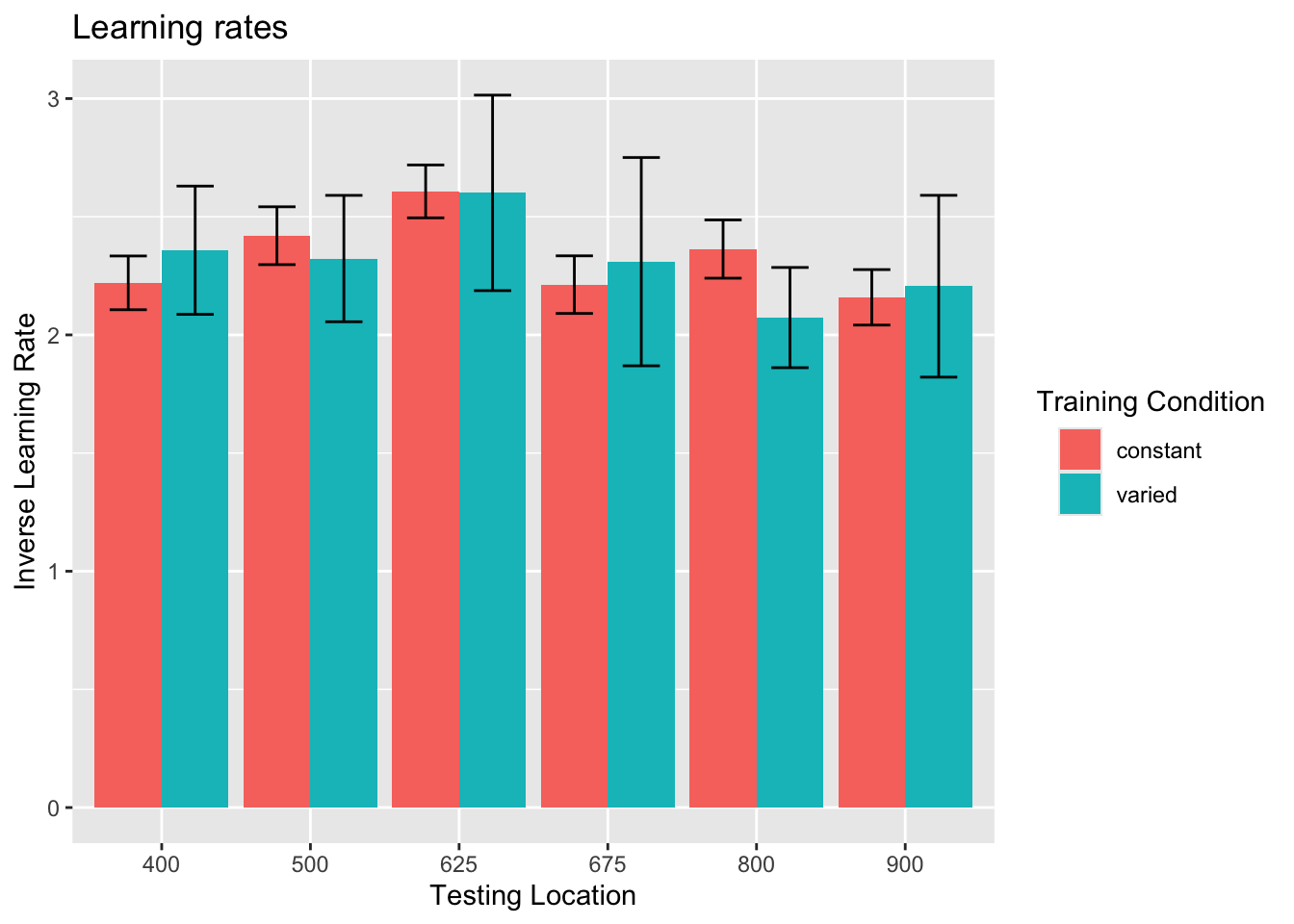
exponential learning models fit to individual subjects

Code
e2TestFits <- readRDS(here::here('data/IGAS-e2TestFits-April4.rds'))
e2TestFits <- e2TestFits %>% mutate(Asymptote.Minus.Start=pAsym-pStart)
exp2.fit2 <- e2TestFits %>% ungroup() %>% group_by(sbjCode,conditType) %>%
  summarise(MeanAsym=mean(pAsym),MeanStart=mean(pStart),
            MeanRate=mean(pRate),
            asymMinusStart=mean(Asymptote.Minus.Start),.groups="keep") %>% 
  ungroup() %>% as.data.frame()

Group comparison of learning rate fits

Code
# mr1=e2TestFits %>% anova_test(dv=pRate,between=conditType,wid=sbjCode,within=positionX,type=3);show(mr1)
# mr2=exp2.fit2 %>% anova_test(dv=MeanRate,between=conditType,wid=sbjCode,type=3);show(mr2) 

# h4<-e2TestFits %>% ggplot(aes(x=positionX,y=pRate,fill=conditType))+geom_bar(stat="summary",position=dodge,fun="mean")+ stat_summary(fun.data=mean_se,geom="errorbar",position=dodge,width=.5)+ggtitle("Learning rates ")+guides(fill=guide_legend(title="Training Condition"))+theme(legend.title.align=.25)+ylab("Inverse Learning Rate")+xlab("Testing Location")
# h4


# mr1=e2TestFits %>% filter(converged==TRUE)%>% anova_test(dv=pRate,between=conditType,wid=sbjCode,within=positionX,type=3);show(mr1)
# mr2=exp2.fit2 %>% anova_test(dv=MeanRate,between=conditType,wid=sbjCode,type=3);show(mr2) 

h4<-e2TestFits %>%filter(Pval<.4)%>% ggplot(aes(x=positionX,y=pRate,fill=conditType))+geom_bar(stat="summary",position=dodge,fun="mean")+ stat_summary(fun.data=mean_se,geom="errorbar",position=dodge,width=.5)+ggtitle("Learning rates ")+guides(fill=guide_legend(title="Training Condition"))+theme(legend.title.align=.25)+ylab("Inverse Learning Rate")+xlab("Testing Location")
h4

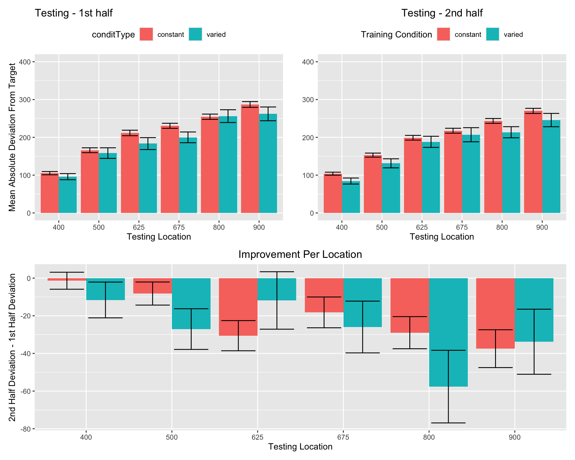
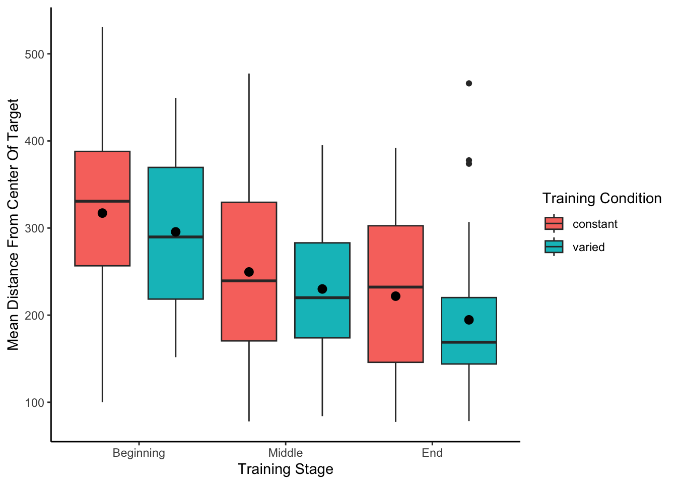
First vs. second half of testing stage

Code
testSplit <- transfer %>%
  group_by(sbjCode, conditType, positionX, testHalfSbj) %>%
  summarise(
    MeanTargetDistance = mean(AbsDistFromCenter),
    MeanScaledDev =mean(scaledDev,trim=.05),
    .groups = "keep"
  ) %>% 
  as.data.frame()

testSplit2 <- transfer %>%
  group_by(sbjCode, conditType, testHalfSbj) %>%
  summarise(
    MeanTargetDistance = mean(AbsDistFromCenter, trim = .01),
    MeanScaledDev =
      mean(scaledDev, trim = .05),
    .groups = "keep"
  ) %>% as.data.frame()


tsw <- testSplit %>% ungroup() %>% 
  pivot_wider(names_from = testHalfSbj,values_from=c(MeanTargetDistance,MeanScaledDev)) %>%
  mutate(endMinusStart = `MeanTargetDistance_2nd-Half` - `MeanTargetDistance_1st-Half`,
    endMinusStartScaled = `MeanScaledDev_2nd-Half` - `MeanScaledDev_1st-Half`) %>% 
    as.data.frame()

tsw2 <- tsw %>% 
  group_by(sbjCode,conditType) %>% summarise(endMinusStart=mean(endMinusStart),endMinusStartScaled=mean(endMinusStartScaled)) %>% as.data.frame()

# testSplit %>% ggplot(aes(x=testHalfSbj,y=MeanTargetDistance))+
#   geom_bar(aes(group=conditType,fill=conditType),stat="summary",position=dodge)+
#   facet_wrap(~positionX,ncol=2)+
#   stat_summary(aes(x=testHalfSbj,group=conditType),fun.data=mean_se,geom="errorbar",position=dodge)


h1=testSplit %>% filter(testHalfSbj=="1st-Half") %>% ggplot(aes(x=positionX,y=MeanTargetDistance))+
 geom_bar(aes(group=conditType,fill=conditType),stat="summary",position=dodge,fun="mean")+stat_summary(aes(x=positionX,group=conditType),fun.data=mean_se,geom="errorbar",position=dodge,width=.8)+
 scale_y_continuous(name="Mean Absolute Deviation From Target",limits=c(0,400))+ 
 ggtitle("Testing - 1st half")+
  ylab("Mean Absolute Deviation From Target")+xlab("Testing Location")+theme(legend.position="top")

h2=testSplit %>% filter(testHalfSbj=="2nd-Half") %>% ggplot(aes(x=positionX,y=MeanTargetDistance))+
 geom_bar(aes(group=conditType,fill=conditType),stat="summary",position=dodge,fun="mean")+
  stat_summary(aes(x=positionX,group=conditType),fun.data=mean_se,geom="errorbar",position=dodge,width=.8) + 
 scale_y_continuous(name="",limits=c(0,400))+ 
 ggtitle("Testing - 2nd half")+
  xlab("Testing Location")+
  theme(plot.title = element_text(hjust = 0.5))+
  theme(legend.position="top") +
  guides(fill=guide_legend(title="Training Condition"))+theme(legend.title.align=.25)

#egg::ggarrange(h1,h2,ncol=2)


h3 <- tsw %>% ggplot(aes(x=positionX,y=endMinusStart))+
  geom_bar(aes(group=conditType,fill=conditType),stat="summary",position=dodge,fun="mean")+
  stat_summary(aes(x=positionX,group=conditType),fun.data=mean_se,geom="errorbar",position=dodge,width=.8)+
  ylab("2nd Half Deviation - 1st Half Deviation")+ 
  ggtitle("Improvement Per Location")+
  xlab("Testing Location")+theme(plot.title = element_text(hjust = 0.5))+
  guides(fill=guide_legend(title="Testing Location")) +theme(legend.position="none")

#ggarrange(h1,h2,h3,h4,ncol=2)

#(h1 + h2) / (h3)

(h1+h2)/h3

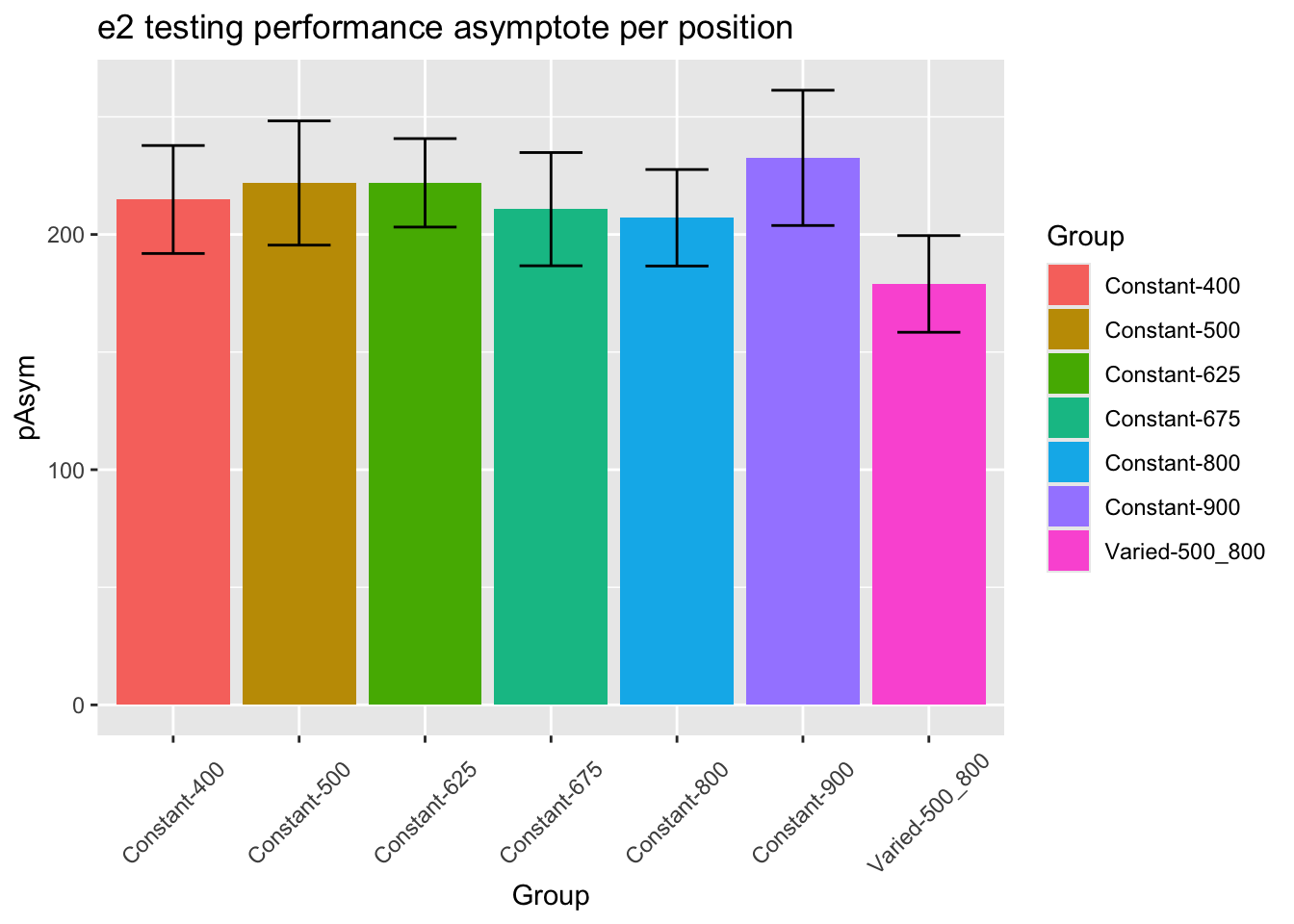
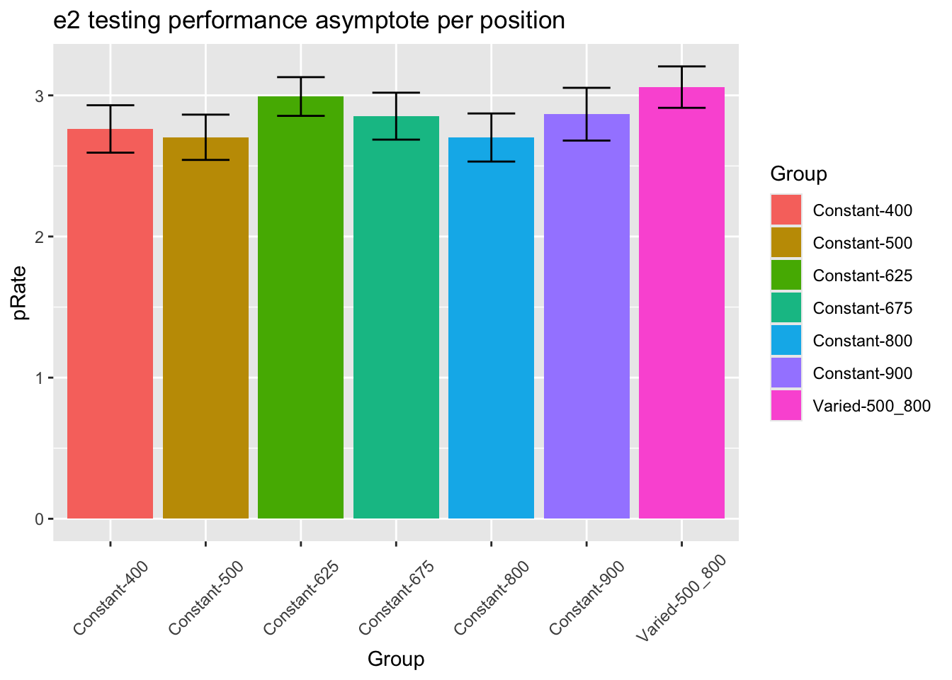
Group Comparison for asymptote-starting performance

Code
# ma1=e2TestFits %>% filter()%>% anova_test(dv=Asymptote.Minus.Start,between=conditType,wid=sbjCode,within=positionX,type=3);show(ma1)
# ma2=exp2.fit2 %>% anova_test(dv=asymMinusStart,between=conditType,wid=sbjCode,type=3);show(ma2) 

e2TestFits %>% ggplot(aes(x=conditType,y=Asymptote.Minus.Start,fill=conditType))+
  geom_bar(stat="summary",position=dodge,fun="mean")+ 
  stat_summary(fun.data=mean_se,geom="errorbar",position=dodge,width=.5)+
  facet_grid(~positionX)+ggtitle("e2 testing (asymptote - start performance)") + 
  theme(axis.text.x = element_text(angle = 45, hjust = 0.5, vjust = 0.5)) 

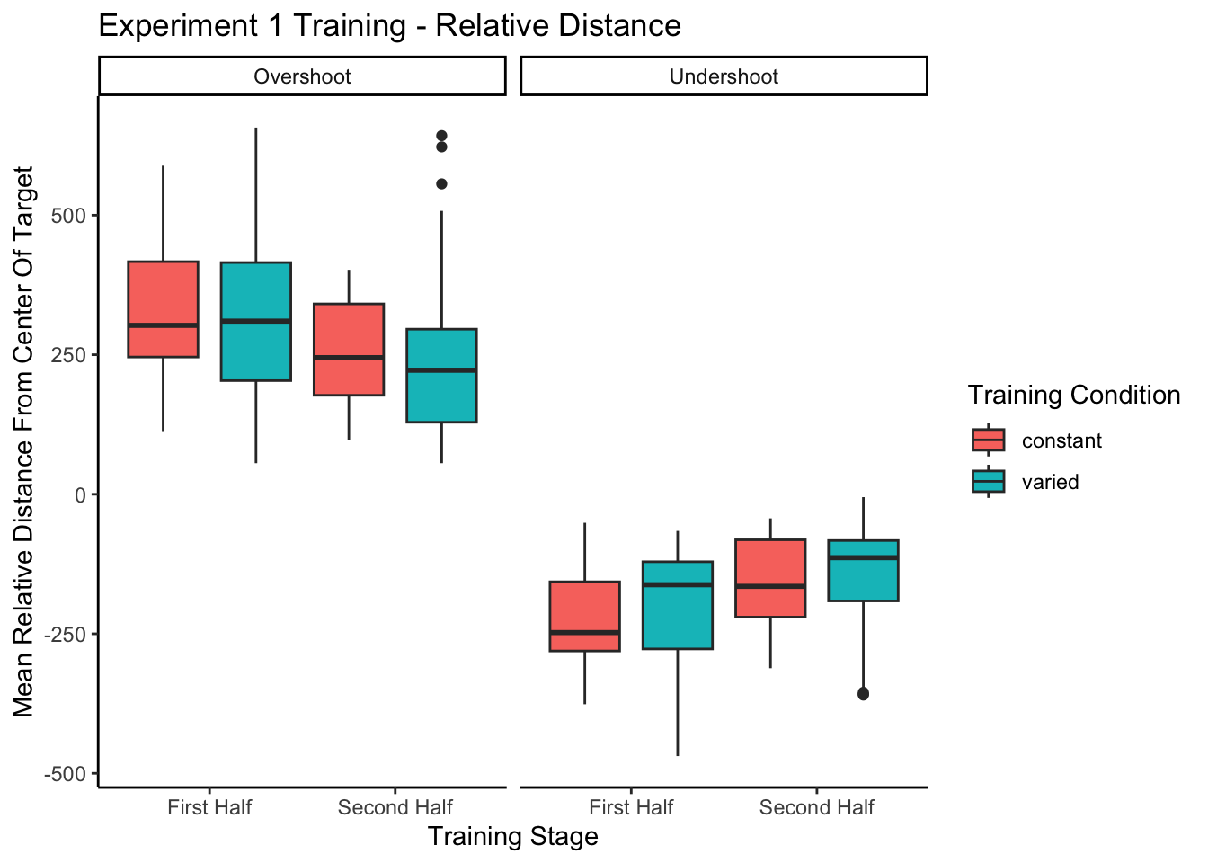
Relative distance and under/overshooting

Reviewer 3 Absolute versus relative distance: From a methodological standpoint, I understand the need to differentiate these two types of distance. However, from a theoretical perspective there may be some issue in differentiating these two concepts. Schema theory relies on relative (or invariant) information to inform the motor program. However, both distances would be important to an instance or exemplar representation. You may want to consider commenting on this issue.

Reviewer 2 For the same reason, the plots showing improvement during training could be due to participants learning the task, rather than fine motor skills. Although task learning and motor learning are impossible to separate cleanly, the common practice in the field is indeed to offer practice trials to reduce the task learning aspects. The authors should address this.

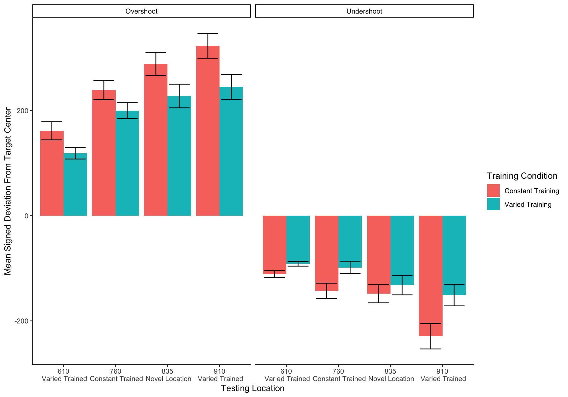
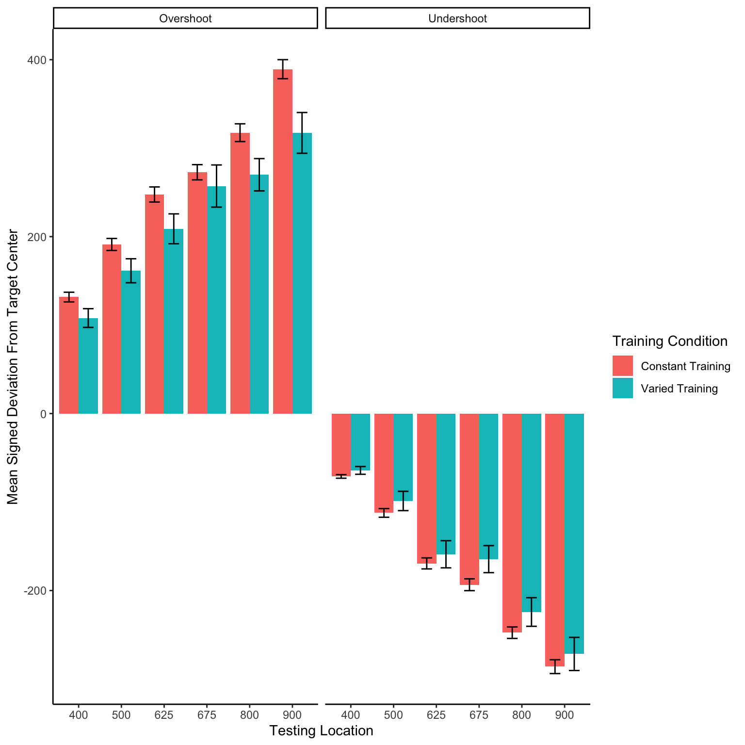
In addition to absolute errors (which is related to variance), the authors should also provide other measures of performance, e.g., the mean of the signed errors, so that readers have a better idea whether there was any meaningful over- or undershooting.

experiment 1 training - relative distances


=========================================================================
conditType devianceDirection      610            760            910      
-------------------------------------------------------------------------
constant       Overshoot                    311.84(307.92)               
constant      Undershoot                    188.05(163.62)               
varied         Overshoot     211.69(234.97)                360.14(322.01)
varied        Undershoot     107.35(81.21)                 244.85(196.47)
-------------------------------------------------------------------------

======================================================
conditType      610           760            910      
------------------------------------------------------
constant                 121.03(269.17)               
varied     39.91(178.12)                150.53(290.04)
------------------------------------------------------

====================================================================
conditType     610           760            835            910      
--------------------------------------------------------------------
constant   7.13(124.02) 107.02(218.49) 142.42(252.34) 122.92(282.58)
varied     3.19(96.67)   92.1(173.9)   103.84(214.4)  108.12(234.59)
--------------------------------------------------------------------

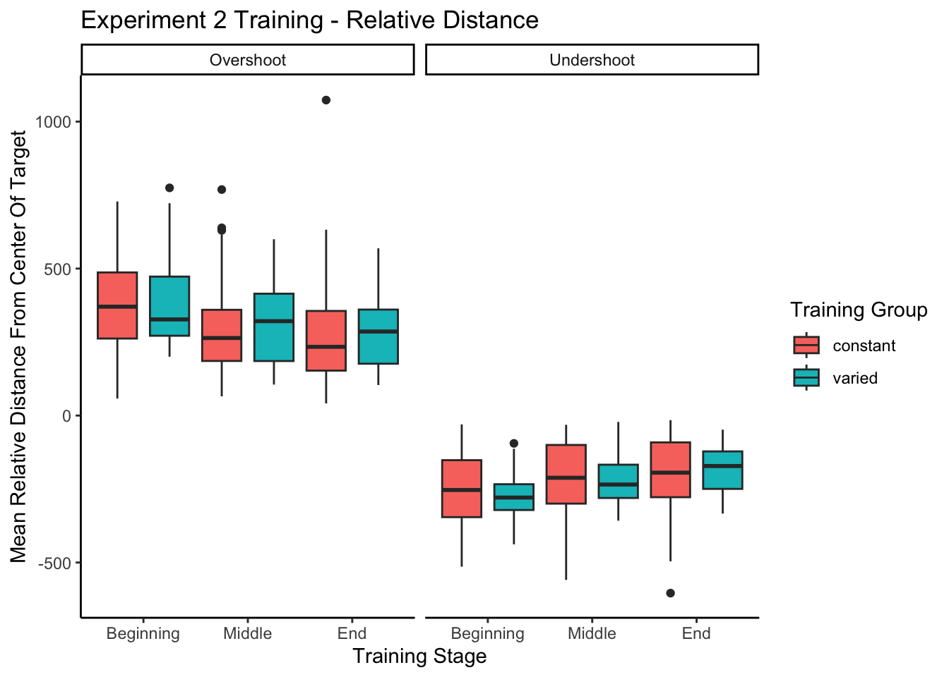
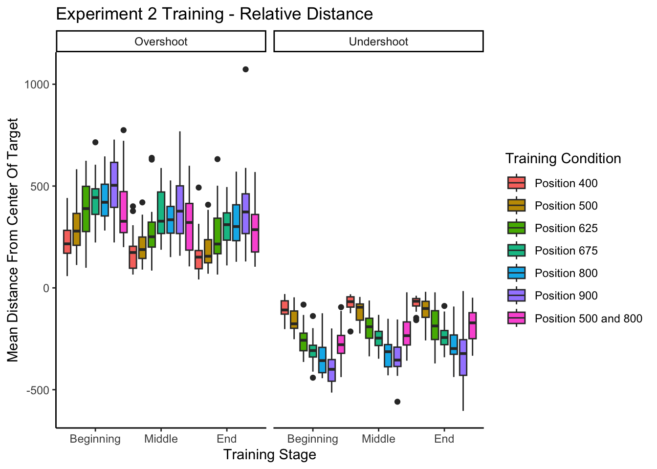
experiment 2 training - relative distances

Experiment 1 Testing - relative distances


====================================================================================================================================
conditType2         msdu_610       msdu_760       msdu_835       msdu_910      msds_610      msds_760      msds_835      msds_910   
------------------------------------------------------------------------------------------------------------------------------------
Constant Training 136.27(84.29) 191.65(112.65) 219.46(139.91) 276.75(153.09) 25.28(158.98) 50.82(217.48) 73.14(250.93) 50.76(313.77)
Varied Training   105.12(51.39)  149.37(93.4)  180.54(129.52) 198.64(137.84) 13.85(116.87) 50.59(169.59) 50.52(217.39) 49.94(237.71)
------------------------------------------------------------------------------------------------------------------------------------

=========================================================================
Condition              610           760           835           910     
-------------------------------------------------------------------------
Constant Training 25.28(158.98) 50.82(217.48) 73.14(250.93) 50.76(313.77)
Varied Training   13.85(116.87) 50.59(169.59) 50.52(217.39) 49.94(237.71)
-------------------------------------------------------------------------

Experiment 2 Testing - relative distances

Experimenet 1 - intermittent testing

Code
intTest.half <- readRDS(here::here("data/e1_intTest.rds"))

intTest.half %>% ggplot(aes(x=positionX,y=MeanTargetDistance))+
  geom_bar(aes(group=trainHalf,fill=trainHalf),stat="summary",fun=mean,position=dodge)+
  facet_wrap(~conditType,ncol=2)+
  stat_summary(aes(x=positionX,group=trainHalf),fun.data=mean_se,geom="errorbar",position=dodge,width=.8)+
  ylab("Mean Distance From Center Of Target")+
  xlab("Intermittent Testing Throw Location")+theme(plot.title = element_text(hjust = 0.5))+
  guides(fill=guide_legend(title="Training Stage"))+theme(legend.title.align=.25)

Code
cnames=c("Condition","610_First Half","760_First Half","910_First Half","610_Second Half","760_Second Half","910_Second Half")
test= intTest.half %>% rename(Condition="conditType") %>% group_by(Condition,trainHalf,positionX) %>% 
  summarise(Mean=round(mean(MeanTargetDistance),2),sd=round(sd(MeanTargetDistance),2)) 
test=test %>% group_by(Condition) %>% mutate(msd=paste(Mean,"(",sd,")",sep="")) %>%
 select(Condition,positionX,trainHalf,msd)%>% pivot_wider(names_from = c(positionX,trainHalf),values_from=c(msd))
test=test %>% as.data.frame()
colnames(test) <- cnames
stargazer(test,type="text",summary=FALSE,rownames=FALSE)

======================================================================================================
Condition 610_First Half 760_First Half 910_First Half 610_Second Half 760_Second Half 910_Second Half
------------------------------------------------------------------------------------------------------
constant  206.64(82.08)  286.51(121.07) 406.93(145.2)   187.2(55.24)    238.21(95.16)  313.27(114.86) 
varied    195.68(78.58)  278.9(105.37)  318.53(134.81)  177.79(70.82)  224.98(108.04)   276.86(110.5) 
------------------------------------------------------------------------------------------------------

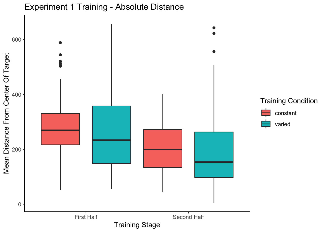
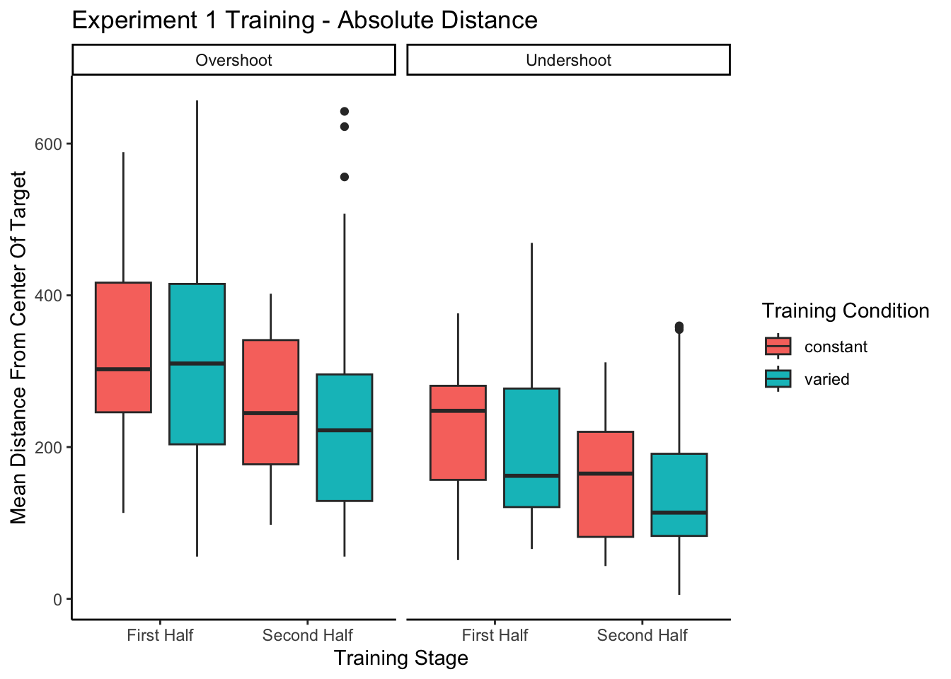
Training plots - Experiment 1

Code
# possible that scaling required loading special package from devtools
exp1Train <- e1 %>% filter(stage!="Transfer",mode==1) %>% group_by(Group,sbjCode) %>%mutate(scaleDev=scale_this(AbsDistFromCenter)) %>%ungroup() %>% group_by(Group,sbjCode,stage,conditType)
exp1Train = exp1Train %>% summarise(MeanTargetDistance=mean(AbsDistFromCenter),scaledDist=mean(scaleDev,trim=.05))
exp1Train$stage <- factor(exp1Train$stage, levels = c("Beginning", "Middle", "End")) #in case the levels get out of order
exp1TrainTrials <- e1 %>% filter(stage!="Transfer",mode==1,trialType!=44) %>% group_by(Group,sbjCode,positionX) %>% mutate(scaleDev=scale_this(AbsDistFromCenter),ind=1,trainIndex=cumsum(ind)) %>%ungroup() %>% group_by(Group,sbjCode,stage,conditType)


# manuscript plot - original
ggplot(data = exp1Train, aes(x=stage, y=MeanTargetDistance)) + geom_boxplot(aes(fill=conditType),position=position_dodge(1))+stat_summary(fun="mean",aes(group=conditType),position=position_dodge(1))+
ylab("Mean Distance From Center Of Target") +xlab("Training Stage")+theme(plot.title = element_text(hjust = 0.5))+guides(fill=guide_legend(title="Training Condition"))+theme(legend.title.align=.5)+theme_classic()

Code
lineplot.CI(data=exp1Train,x.factor=stage,group=conditType,response=scaledDist,xlab="Training Stage",x.leg=2,legend=TRUE,ylab="Distance from Target (scaled)",main="Training Performance - Experiment 1",col=c("red","black"))

Code
lineplot.CI(data=exp1Train,x.factor=stage,group=conditType,response=MeanTargetDistance,xlab="Training Stage",x.leg=2,legend=TRUE,ylab="Distance From Target",main="Training Performance - Experiment 1",col=c("red","blue"))

Not in manuscript

fit to testing performance averaged across positions

Code
e2Fits.AggPos <- readRDS(here::here('data/IGAS-e2Fits.AggPos-April_12.rds'))

e2Fits.AggPos %>% ggplot(aes(x=Group,y=pStart,fill=Group))+
  geom_bar(stat="summary",position=dodge,fun="mean")+ 
  stat_summary(fun.data=mean_se,geom="errorbar",position=dodge,width=.5)+
  ggtitle("experiment 2 - starting performance per position") + 
  theme(axis.text.x = element_text(angle = 45, hjust = 0.5, vjust = 0.5)) 

Code
e2Fits.AggPos %>% ggplot(aes(x=Group,y=pAsym,fill=Group))+
  geom_bar(stat="summary",position=dodge,fun="mean")+ 
  stat_summary(fun.data=mean_se,geom="errorbar",position=dodge,width=.5)+
  ggtitle("e2 testing performance asymptote per position ") +
  theme(axis.text.x = element_text(angle = 45, hjust = 0.5, vjust = 0.5)) 

Code
e2Fits.AggPos %>% ggplot(aes(x=Group,y=pRate,fill=Group))+
  geom_bar(stat="summary",position=dodge,fun="mean")+ 
  stat_summary(fun.data=mean_se,geom="errorbar",position=dodge,width=.5)+
  ggtitle("e2 testing performance asymptote per position ") +
  theme(axis.text.x = element_text(angle = 45, hjust = 0.5, vjust = 0.5)) 

Code
#mr1=e2Fits.AggPos %>% anova_test(dv=pRate,between=conditType,wid=sbjCode,type=3);show(mr1)

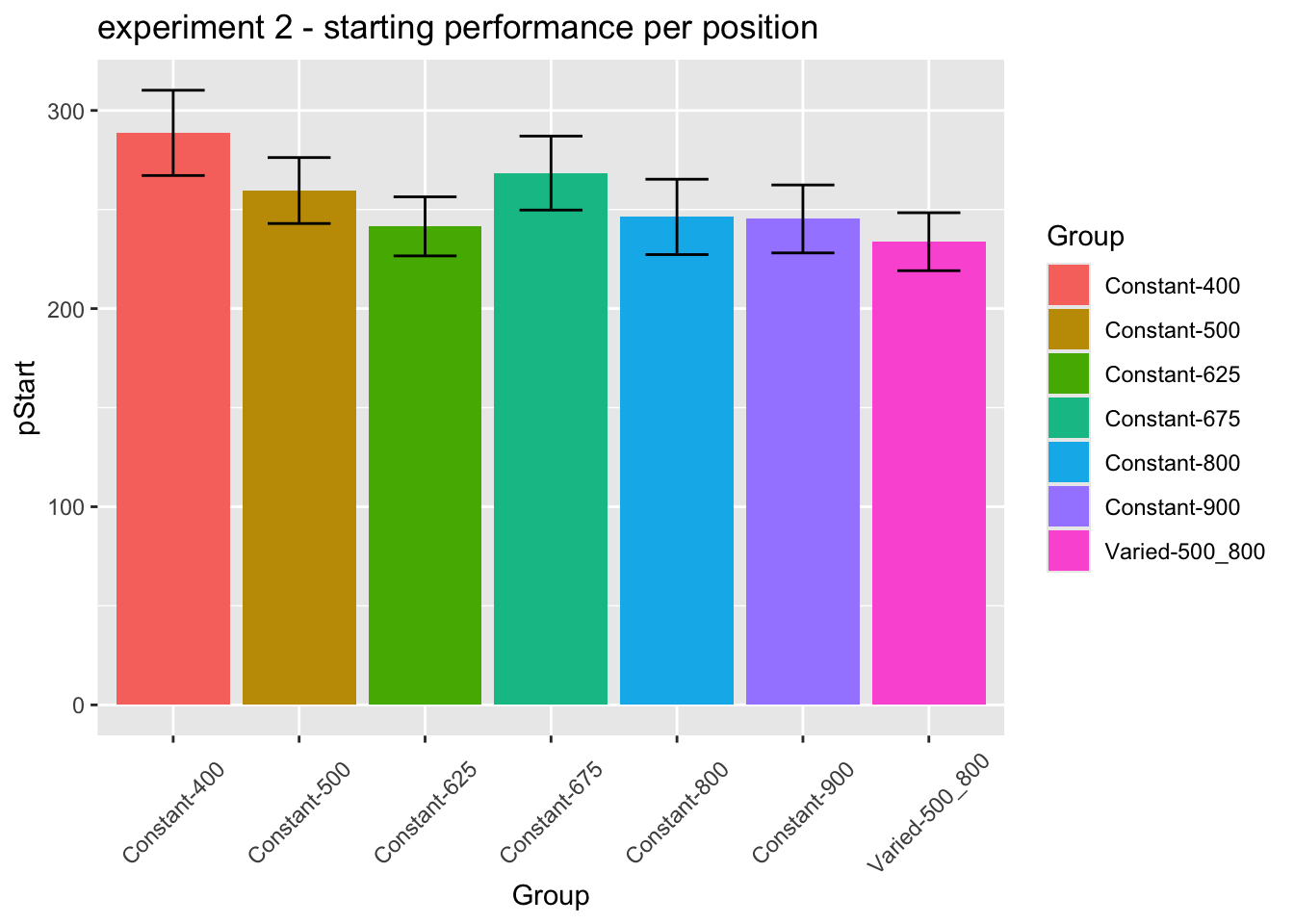
statistical tests for starting performance

Code
ms1=e2TestFits %>% filter(converged==TRUE) %>% anova_test(dv=pStart,between=conditType,wid=sbjCode,within=positionX,type=3);
ms2=exp2.fit2 %>% anova_test(dv=MeanStart,between=conditType,wid=sbjCode,type=3);
#ms1
ms2 
ANOVA Table (type III tests)

      Effect DFn DFd    F     p p<.05   ges
1 conditType   1 206 3.04 0.083       0.015
Code
e2TestFits %>% ggplot(aes(x=conditType,y=pStart,fill=conditType))+
  geom_bar(stat="summary",position=dodge,fun="mean")+ 
  stat_summary(fun.data=mean_se,geom="errorbar",position=dodge,width=.5)+
  facet_grid(~positionX)+ggtitle("experiment 2 - starting performance per position") + 
  theme(axis.text.x = element_text(angle = 45, hjust = 0.5, vjust = 0.5)) 

statistical tests for asymptote

Code
ma1=e2TestFits %>% filter(converged==TRUE)%>% anova_test(dv=pAsym,between=conditType,wid=sbjCode,within=positionX,type=3);
ma2=exp2.fit2 %>% anova_test(dv=MeanAsym,between=conditType,wid=sbjCode,type=3);
ma2
ANOVA Table (type III tests)

      Effect DFn DFd    F     p p<.05   ges
1 conditType   1 206 3.38 0.067       0.016
Code
e2TestFits %>% ggplot(aes(x=conditType,y=pAsym,fill=conditType))+
  geom_bar(stat="summary",position=dodge,fun="mean")+ 
  stat_summary(fun.data=mean_se,geom="errorbar",position=dodge,width=.5)+
  facet_grid(~positionX)+ggtitle("e2 testing performance asymptote per position ") + 
  theme(axis.text.x = element_text(angle = 45, hjust = 0.5, vjust = 0.5)) 

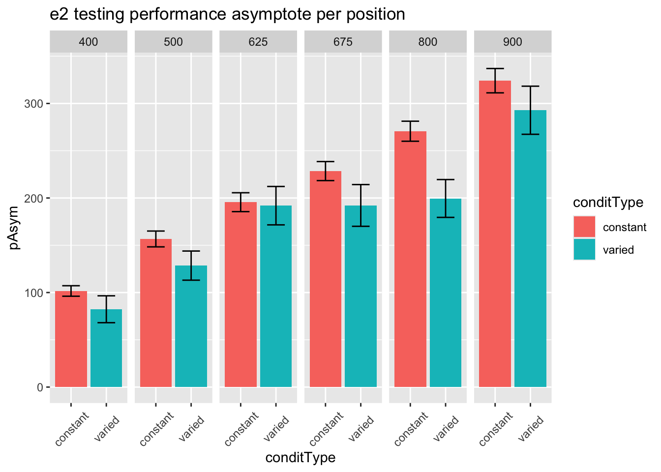
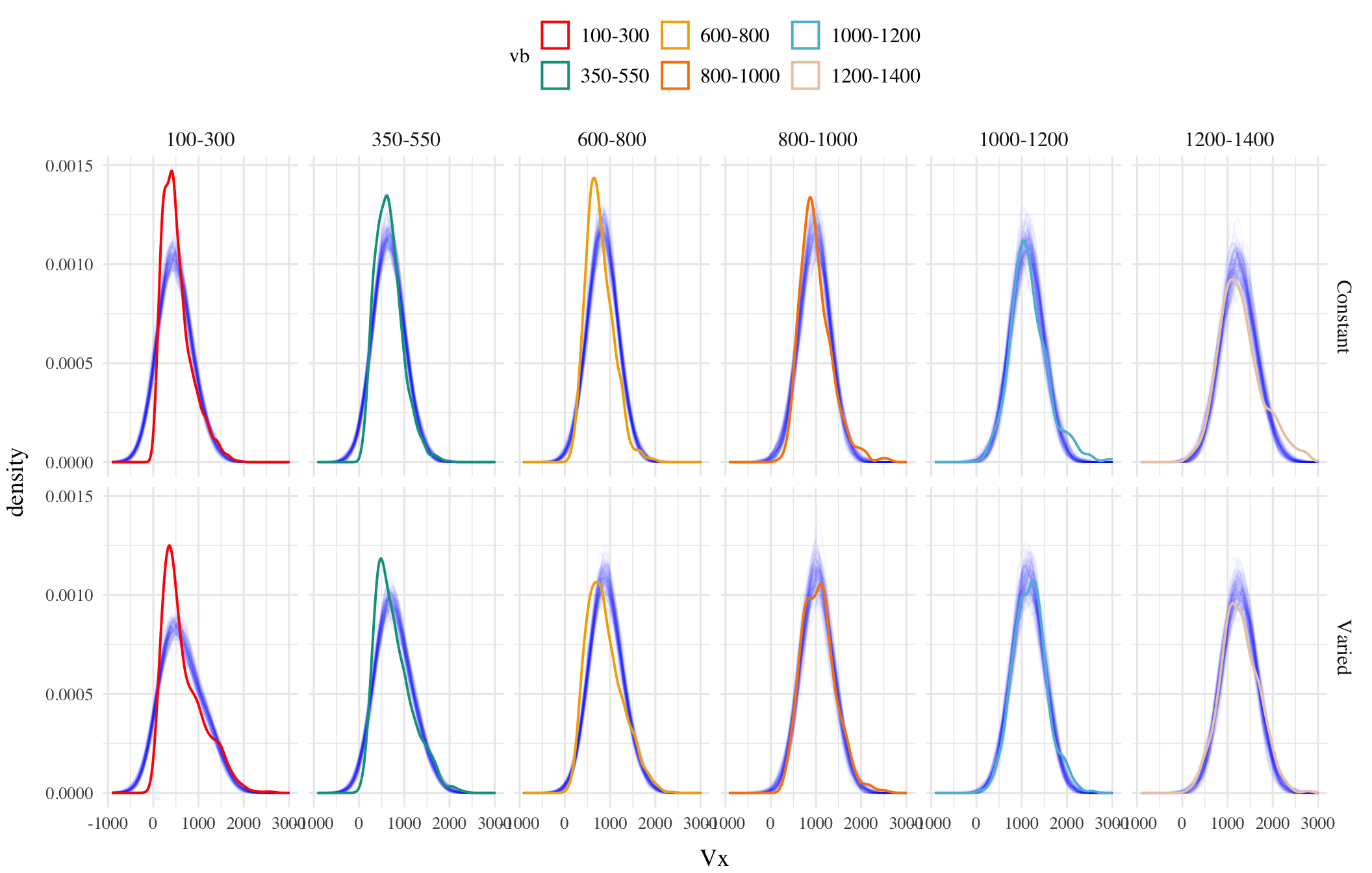
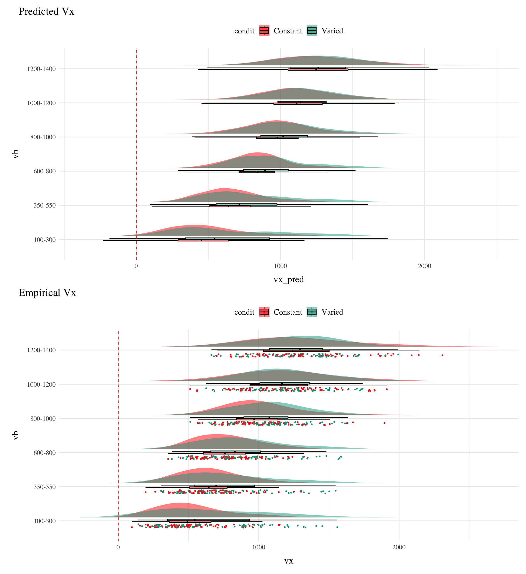
Appendix - Project 2 - Experiment 1

Code
# print(getwd())
# here::set_here(path='..')
# print(getwd())
#source(here::here("Functions", "packages.R"))
pacman::p_load(dplyr,purrr,tidyr,tibble,ggplot2,
  brms,tidybayes, rstanarm,emmeans,broom,bayestestR,
  stringr, here,conflicted, patchwork, knitr, cowplot, RColorBrewer,data.table,gt,
  ggh4x,htmltools,future,furrr,ez)
walk(c("dplyr","here"), conflict_prefer_all, quiet = TRUE)

walk(c("Display_Functions", "org_functions", "Table_Functions"), ~ source(here::here(paste0("Functions/", .x, ".R"))))
Code
test <- readRDS(here::here("data/e1_08-21-23.rds")) |> filter(expMode2 == "Test")  |>
  select(id,condit,bandInt,vb,vx,dist,sdist,bandType,tOrder)

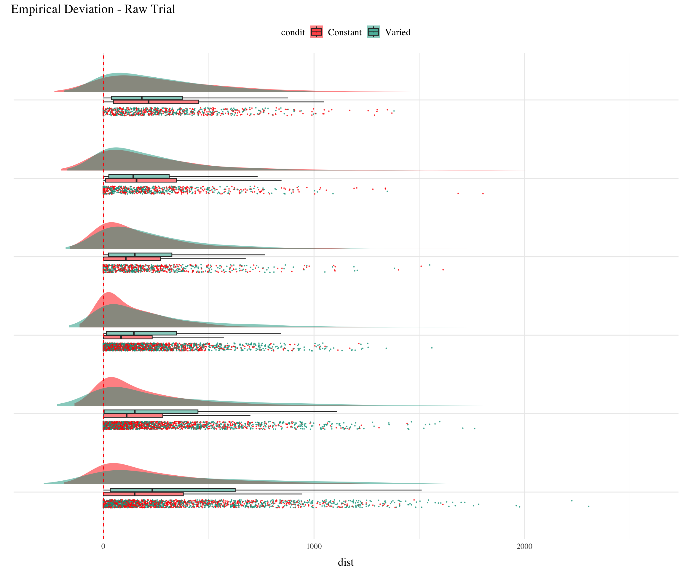
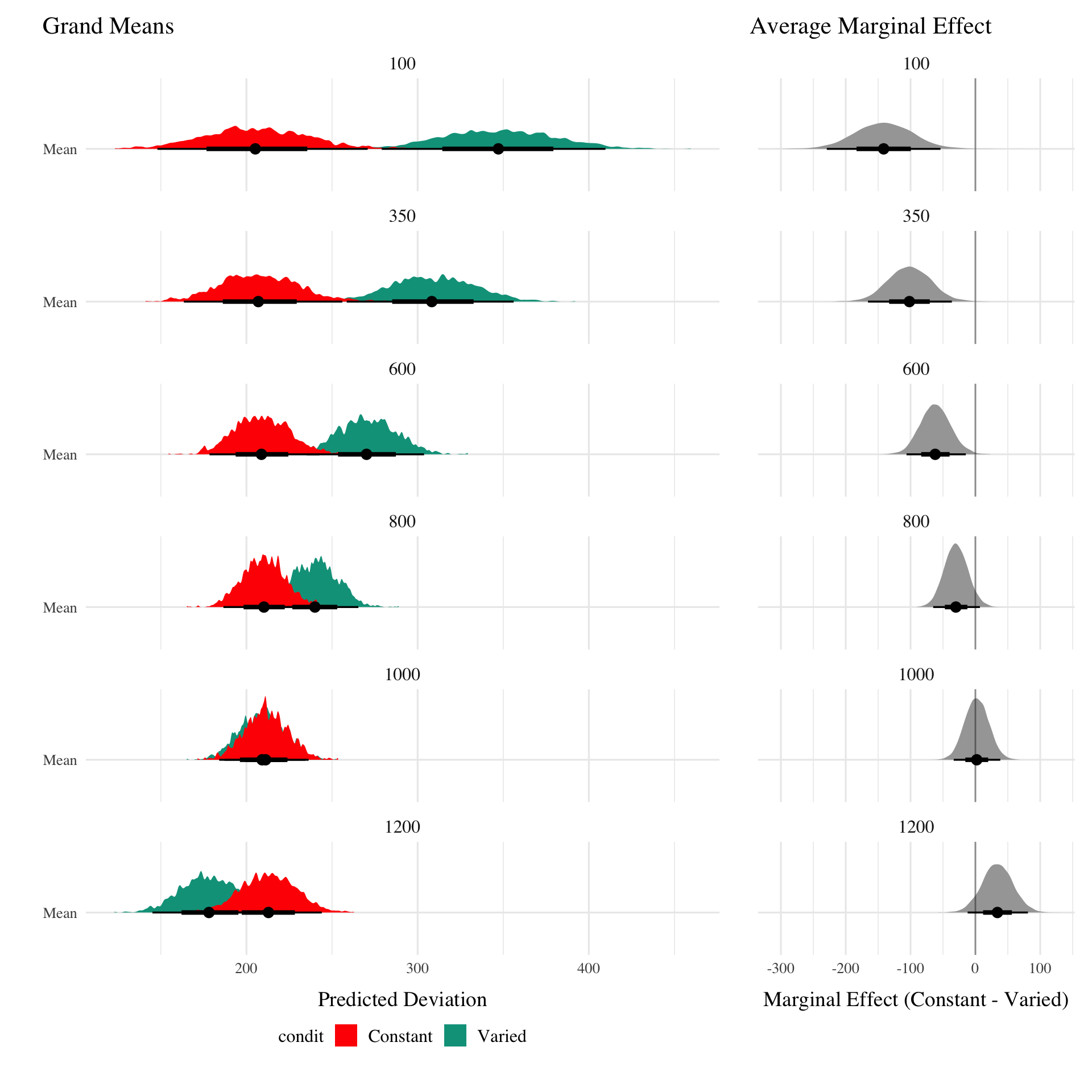
Posterior Predictive Distributions

Code
dist_pred <- 
  posterior_predict(e1_distBMM, ndraws = 500) |> 
  array_branch(margin=1) |> 
   map_dfr( 
    function(yrep_iter) {
      test  |>
        mutate(dist_pred = yrep_iter)
    },
    .id = 'iter'
  ) |>
  mutate(iter = as.numeric(iter))


dist_pred  |>
  filter(iter < 100) %>%
  ggplot(aes(dist_pred, group = iter)) +
  geom_line(alpha = .03, stat = 'density', color = 'blue') +
  geom_density(data = test,
               aes(dist,col=vb),
               inherit.aes = FALSE,
               size = 0.7) + # 1
  facet_grid(condit ~ vb) +
  xlab('Deviation')
Figure 1: Posterior Predictive distributions for Absolute Deviance. Posterior Draws in Blue, colored lines are empirical data.
Code
vx_pred <- 
  posterior_predict(e1_vxBMM, ndraws = 500) |> 
  array_branch(margin=1) |> 
   map_dfr( 
    function(yrep_iter) {
      test  |>
        mutate(vx_pred = yrep_iter)
    },
    .id = 'iter'
  ) |>
  mutate(iter = as.numeric(iter))


vx_pred  |>
  filter(iter < 100) %>%
  ggplot(aes(vx_pred, group = iter)) +
  geom_line(alpha = .03, stat = 'density', color = 'blue') +
  geom_density(data = test,
               aes(vx,col=vb),
               inherit.aes = FALSE,
               size = 0.7) + # 1
  facet_grid(condit ~ vb) +
  xlab('Vx')
Figure 2: Posterior Predictive distributions for Vx. Posterior Draws in Blue, colored lines are empirical data.

Empirical vs. Predicted

Code
{
vx_pred  |>
  filter(iter < 100)  |> group_by(id,condit,vb,iter) |>
  summarise(vx_pred=mean(vx_pred)) %>%
  ggplot(aes(x=vb,y=vx_pred,fill=condit)) + 
  geom_flat_violin( position = position_nudge(x = 0.1, y = 0),
                   adjust = 1.5,
                   trim = FALSE, alpha = .5, colour = NA) +
  # geom_point(aes(x = as.numeric(vb) - 0.15, y = vx_pred, colour = vb),
  #            position = position_jitter(width = 0.05, height = 0),
  #            size = 1, shape = 20) +
  geom_boxplot(aes(x = vb, y = vx_pred, fill = condit),
               outlier.shape = NA,
               alpha = 0.5,
               width = 0.1,
               colour = "black") +
  geom_hline(yintercept = 0,
             linetype = 'dashed',
             color = 'red',
             size = 0.4) + 
  coord_flip() + ggtitle("Predicted Vx")  
} / {
vx_pred  |>
  filter(iter < 2)  |> group_by(id,condit,vb) |>
  summarise(vx=mean(vx)) %>%
  ggplot(aes(x=vb,y=vx,fill=condit)) + 
  geom_flat_violin( position = position_nudge(x = 0.1, y = 0),
                   adjust = 1.5,
                   trim = FALSE,
                   alpha = .5,
                   colour = NA) +
  geom_point(aes(x = as.numeric(vb) - 0.15,col=condit),
             # position = position_jitter(width = 0.05),
             position = position_jitter(width = 0.05, height = 0),
             size = 1,
             shape = 20) +
  geom_boxplot(
               outlier.shape = NA,
               alpha = 0.5,
               width = 0.1,
               colour = "black") +
  geom_hline(yintercept = 0,
             linetype = 'dashed',
             color = 'red',
             size = 0.4) + 
  coord_flip() + ggtitle("Empirical Vx") 
}
Figure 3: Bayesian Mixed Model predictions vs. Empirical Predictions - X velocity

Different Aggregations

Code
epId <- dist_pred  |>
  filter(iter < 2)  |> group_by(id,condit,vb) |>
  summarise(dist=median(dist)) |>
  ggplot(aes(x=vb,y=dist,fill=condit)) + 
  geom_flat_violin(aes(fill=condit), position = position_nudge(x = 0.1, y = 0),
                   adjust = 1.5,trim = FALSE, alpha = .5, colour = NA) +
  geom_point(aes(x = as.numeric(vb) - 0.15, col=condit),
             position = position_jitter(width = 0.05, height = 0),
             size = 1, shape = 20, alpha=.7) +
  geom_boxplot(aes(x=vb,y=dist,fill=condit),
               outlier.shape = NA,
               alpha = 0.5, width = 0.1) +
  geom_hline(yintercept = 0,
             linetype = 'dashed',
             color = 'red',
             size = 0.4) + 
  coord_flip() + ggtitle("Empirical Deviation - Subject level averaging") 


epId 
Figure 4: E1. Distribution of Vx at Participant level
Code
epTrial <- dist_pred  |>
  filter(iter < 2)  |> group_by(id,condit,vb) |>
  ggplot(aes(x=vb,y=dist,fill=condit)) + 
  geom_flat_violin(aes(fill=condit), position = position_nudge(x = 0.1, y = 0),
                   adjust = 1.5,trim = FALSE, alpha = .5, colour = NA) +
  geom_point(aes(x = as.numeric(vb) - 0.15, col=condit),
             position = position_jitter(width = 0.05, height = 0),
             size = .5, shape = 20, alpha=.7) +
  geom_boxplot(aes(x=vb,y=dist,fill=condit),
               outlier.shape = NA,
               alpha = 0.5, width = 0.1) +
  geom_hline(yintercept = 0,
             linetype = 'dashed',
             color = 'red',
             size = 0.4) + 
  coord_flip() + ggtitle("Empirical Deviation - Raw Trial") +
   theme(axis.title.y=element_blank(),
        axis.text.y=element_blank())

epTrial
Figure 5: E1. Distribution of Vx at Trial level
Code
new_data_grid=map_dfr(1, ~data.frame(unique(test[,c("id","condit","bandInt")])))

cSamp <- e1_distBMM  |> 
  emmeans("condit",by="bandInt",at=list(bandInt=c(100,350,600,800,1000,1200)),
          epred = TRUE, re_formula = NA) |> 
  pairs() |> gather_emmeans_draws()  |>
  group_by(contrast, .draw,bandInt) |> summarise(value=mean(.value), n=n())


 ameBand <- cSamp |> ggplot(aes(x=value,y="")) + 
  stat_halfeye() + 
  geom_vline(xintercept=0,alpha=.4)+
  facet_wrap(~bandInt,ncol=1) + labs(x="Marginal Effect (Constant - Varied)", y= NULL)+
  ggtitle("Average Marginal Effect")

bothConditGM <- e1_distBMM %>%
  epred_draws(newdata = new_data_grid,ndraws = 2000, re_formula = NA) |>
  ggplot(aes(x=.epred,y="Mean",fill=condit)) + 
  stat_halfeye() +facet_wrap(~bandInt, ncol = 1) +
  labs(x="Predicted Deviation", y=NULL)+
  ggtitle("Grand Means") +theme(legend.position = "bottom")

(bothConditGM | ameBand) + plot_layout(widths=c(2,1.0))
Figure 6: E1. Predicted Means Per Condition and Band, and Average Marginal Effect (Constant - Varied)

:::