The Role of Variability in Learning Generalization: A Computational Modeling Approach
Indiana University
May 28, 2024
Learning Generalization
- Learning is often specific
- Longstanding scientific interest in how to improve generalization or transfer
Variability
- Variation during training linked to improved transfer in numerous domains
- Category learning, perceptual learning, education, visuomotor learning
- sometimes alternatively termed diversity, heterogenity, numerosity etc.
- What does variability mean in the context of learning interventions?
- How spread out examples are in the task space
- The number of unique items/problems experienced
- exposure to wider array of contexts/background conditions
Common Empirical Patterns
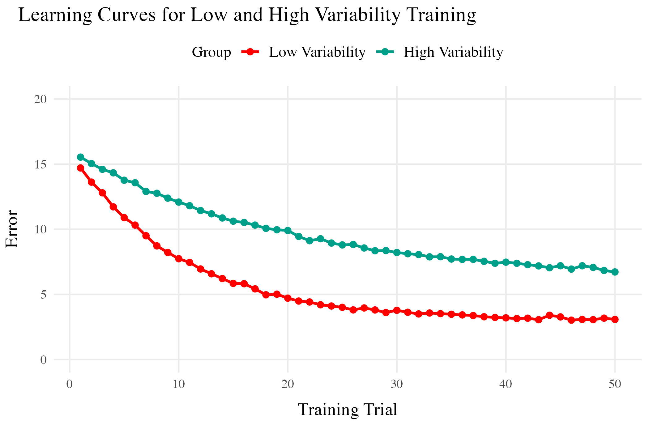
Training
- Both training conditions complete the same number of training trials.
- Varied group has worse training performance.
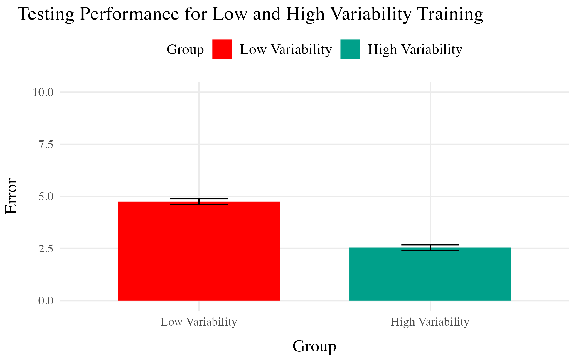
Testing
- Tested from novel conditions.
- Varied group has better test performance
But also plenty of contradictory results and complications
- Cases where varied training doesn’t benefit generalization
- Cases where more training variation results in worse outcomes
- Cases where the influence of variation interacts with some other factor
- difficulty
- prior knowledge
- Frequency effects, or amount of training/learning before testing
Overview
Project 1
- Visuomotor projectile launching task
- two experiments
- Beneficial effect of variability
- Instance-based similarity model
Project 2
- Visuomotor extrapolation task
- Three experiments
- Effect of variability is null or negative
- Connectionist model (ALM) and hybrid associative & rule model (EXAM)
Project 1
An instance-based model account of the benefits of varied practice in visuomotor skill1
Theoretical Frameworks
- Desirable Difficulties Framework (Bjork & Bjork, 2011)
- Challenge Point Framework (Guadagnoli & Lee, 2004)
- Schema Theory (Schmidt, 1975)
Issues with previous research
- Assumptions about what is encoded
- Assumptions about the formation of abstractions
- Aggregation issues and similarity confounds
Designs that avoid similarity issue
Kerr & Booth 1978
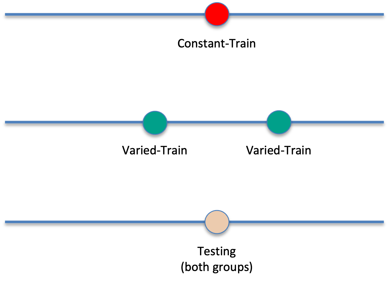
- Bean bag tossing task
- Constant and varied conditions train from distinct positions
- Both groups are tested from the position where the constant group trained
- Impressive demonstration of varied training outperforming constant training
Kerr & Booth (1978)
Experiment 1
- Conceptual replication of Kerr & Booth design
- Also test positions novel to both groups
- Validate computerized visuomotor learning task
Experiment 1 Design
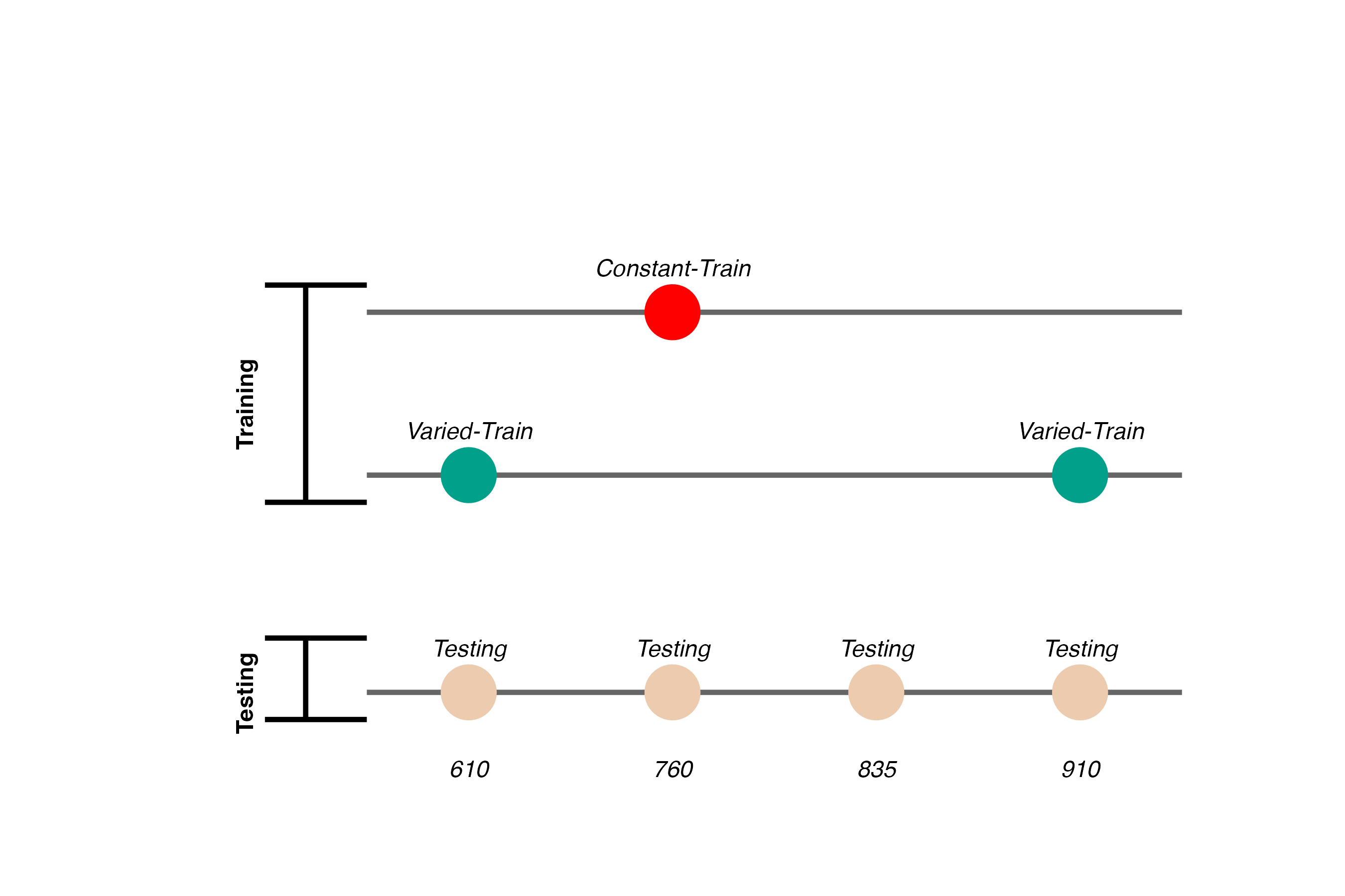
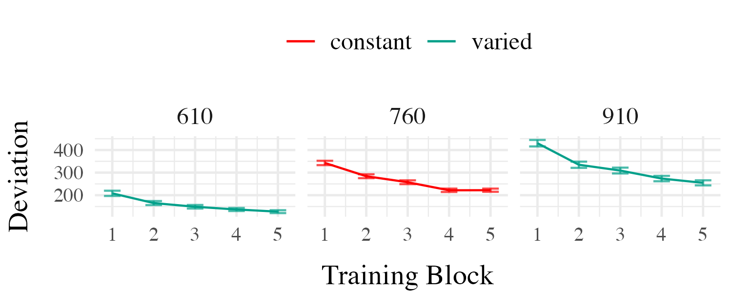
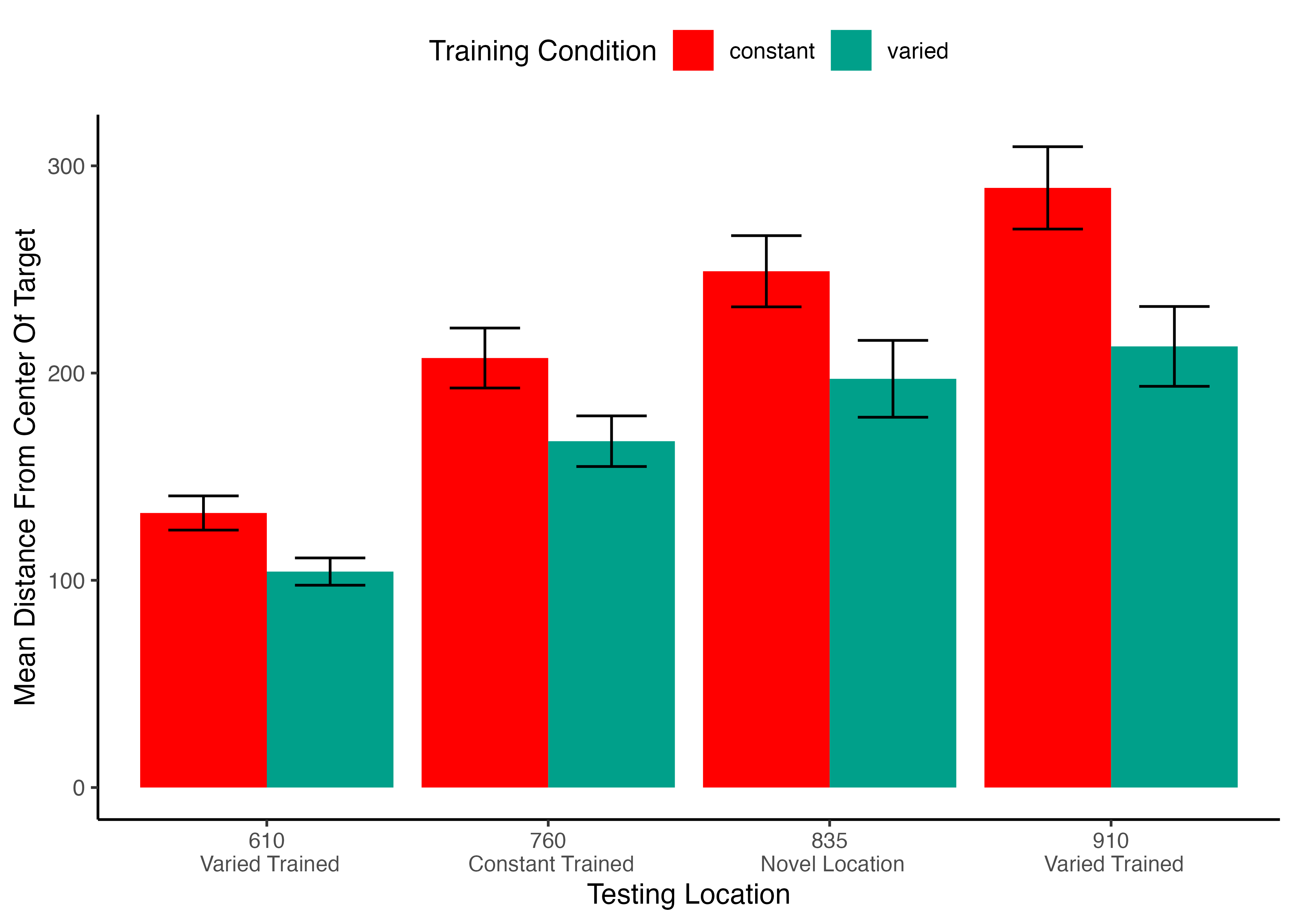
- Constant trains from one position (760)
- 200 trials
- Varied trains from two positions (610 and 910)
- 100 trials per position
- Both groups are tested from all three training positions, and a new position novel to both groups (835)
Hit The Target Task
- Training Stage - 200 training trials with feedback. Constant groups trains from single position. Varied group practices from two positions.
- Transfer Stage - All subjects tested from both positions they were trained, and the positions trained by other group
- Data recorded - For every throw, recorded the X velocity and Y velocity of ball at release
Project 1 - Experiment 1 Results
Training
Testing
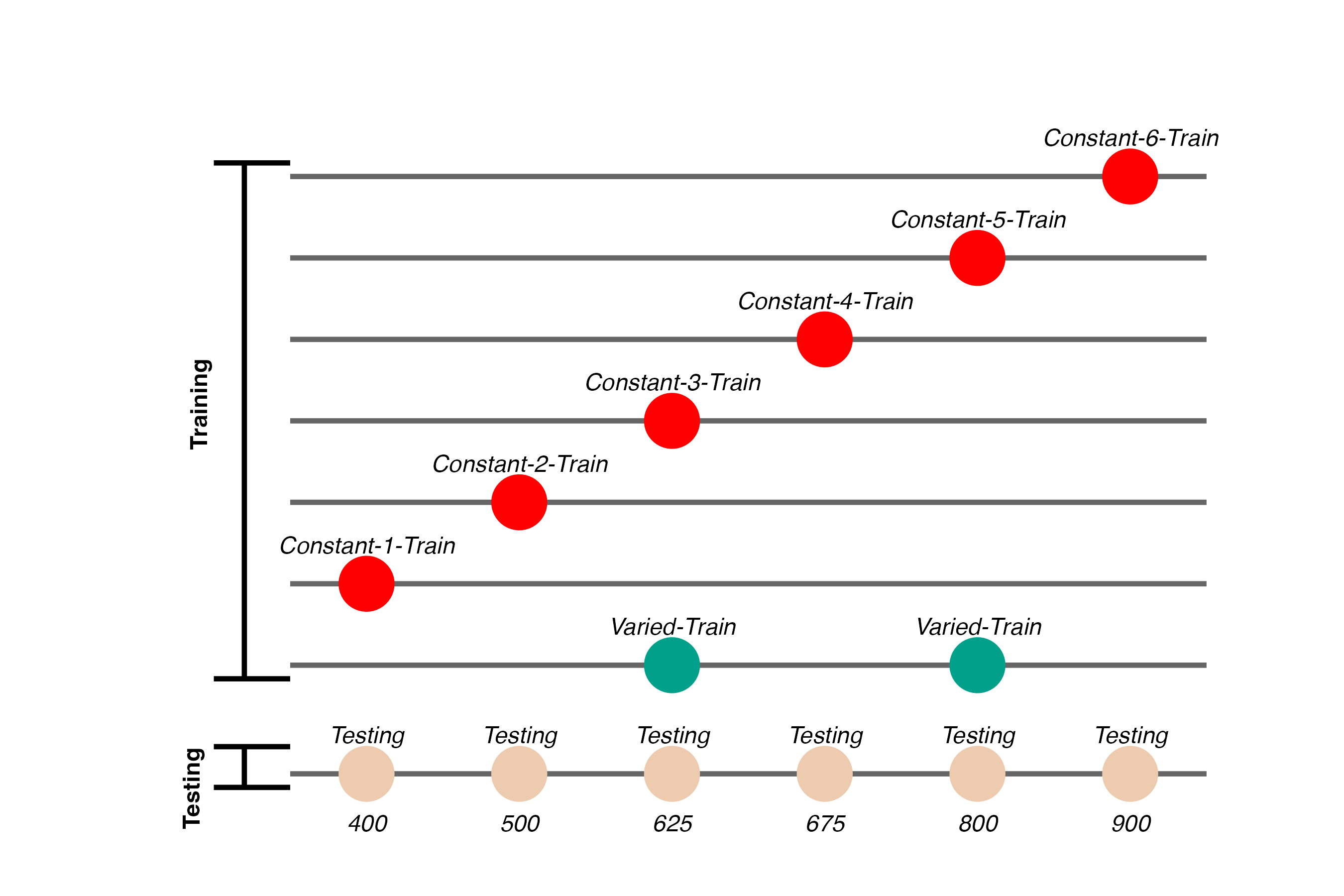
Experiment 2 Design
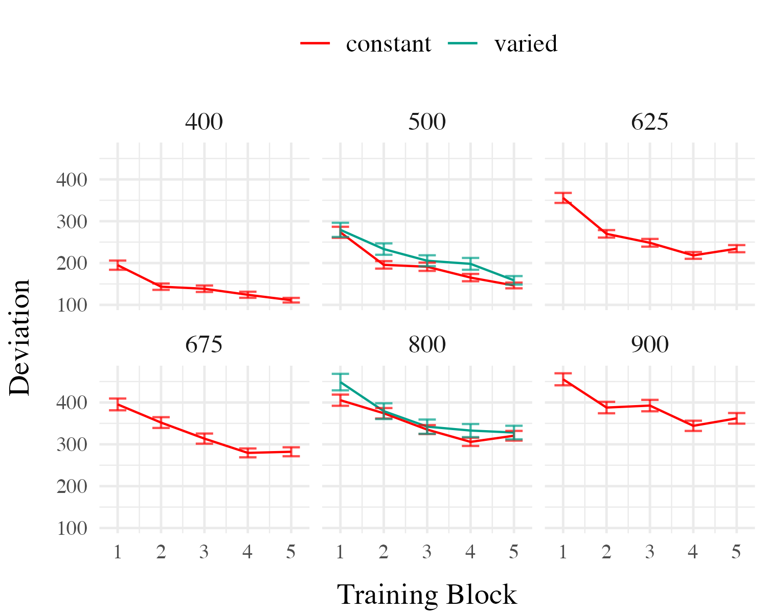
Project 1 - Experiment 2 Results
Training
Testing
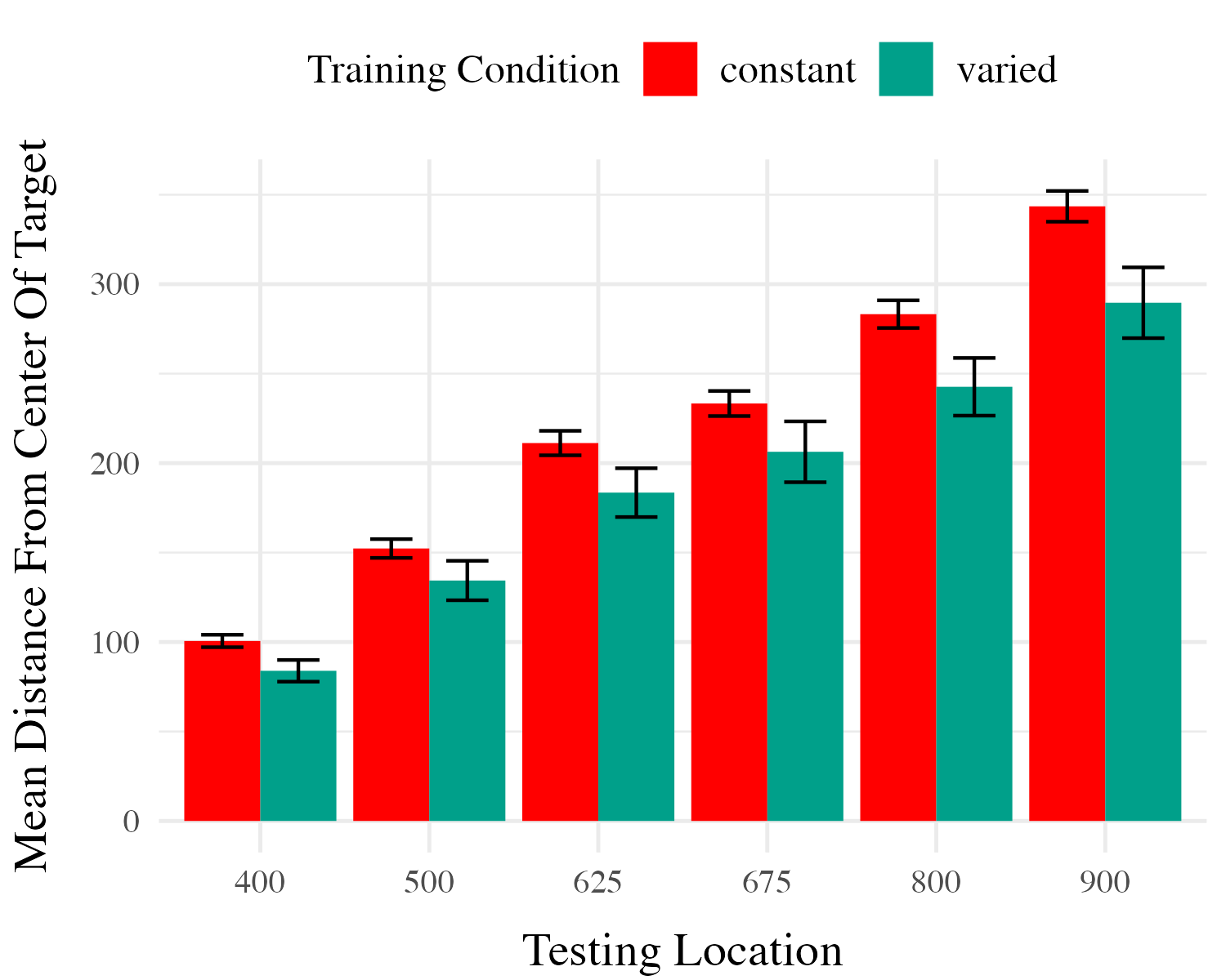
Project 1 Computational Model
Instance encoding, and similarity-based generalization assumptions
- Instances refers to individual throws (x and y velocity)
- Similarity refers to the distance between training throws and the solution space of each of the eventual testing positions.
Project 1 Computational Model
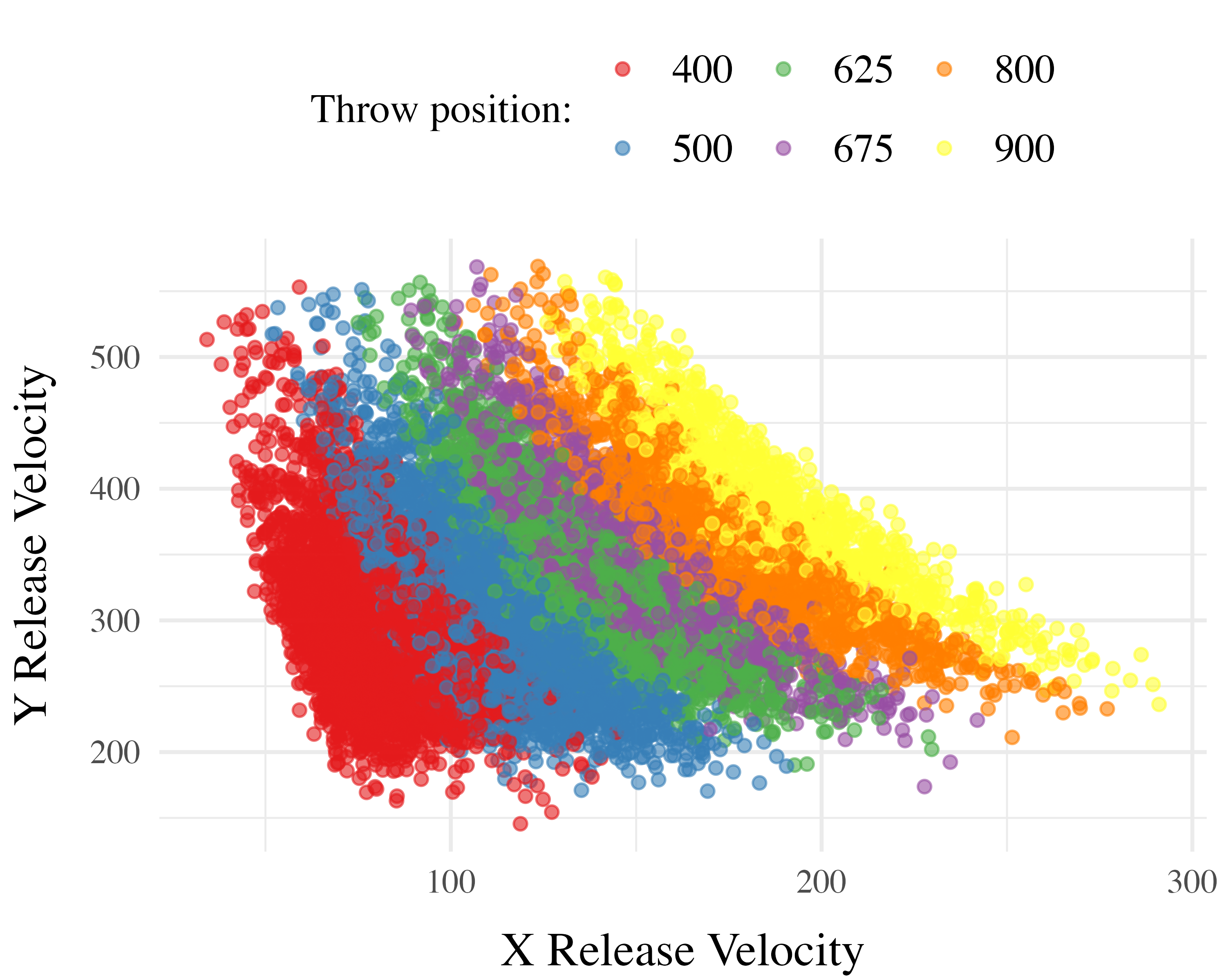
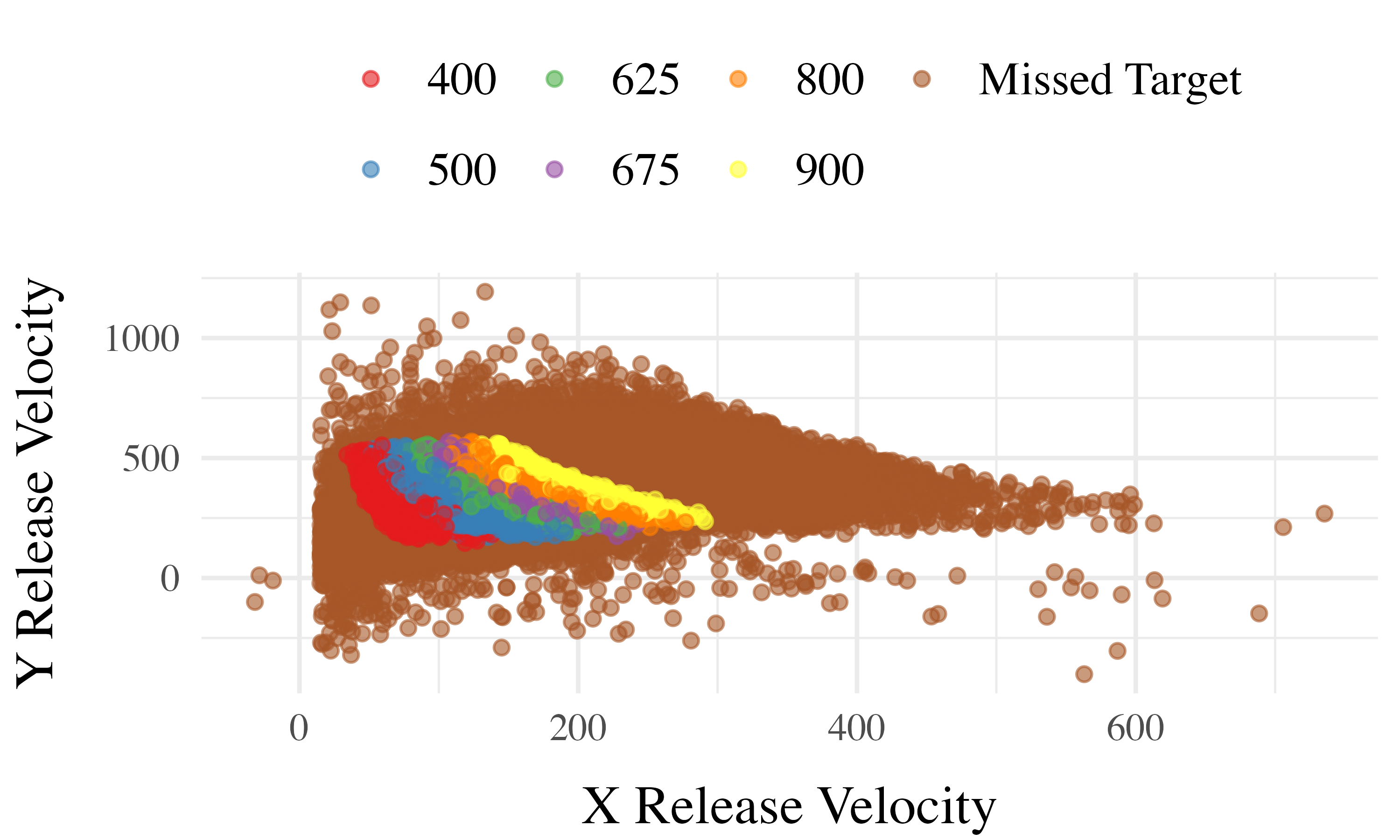
Computing Similarity
- Euclidean distance between each training throw, and each solution space
- Similarity computed as a Gaussian decay function of distance, i.e. larger distances result in lower similarity
- Each participant gets their own similarity score for each of the 6 testing positions
- similarity score for a given testing position is the sum of the similarities between each training throw and the entire empirical solution space
Model Definition
- \(d_{i,j} = \sqrt{(x_{Train_i}-x_{Solution_j})^2 + (y_{Train_i}-y_{Solution_j})^2 }\)
- \(Similarity_{I,J} = \sum_{i=I}\sum_{j=J} (e^{-c^\cdot d^{p}_{i,j}})\)
Non-linear similarity
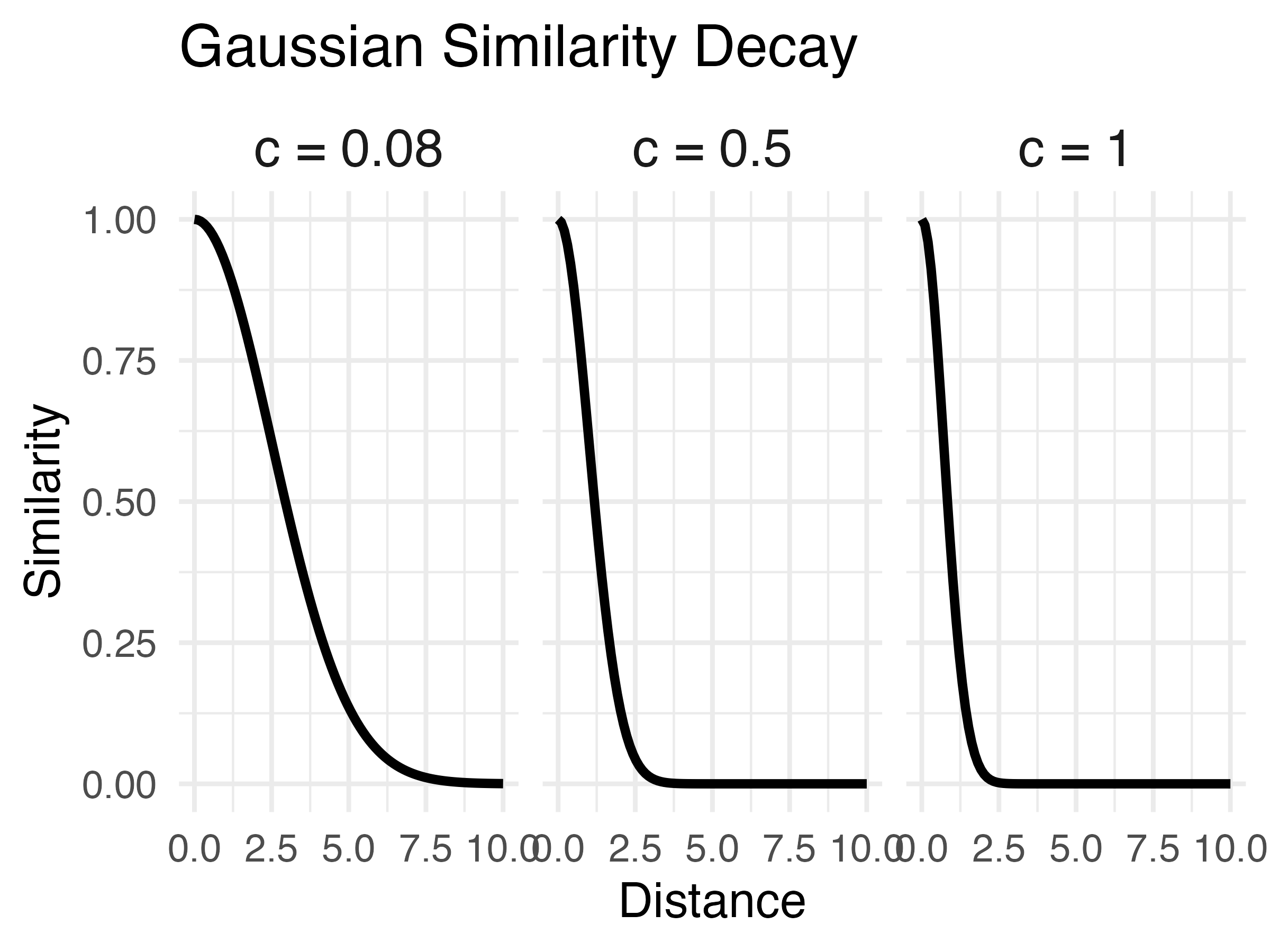
Does this similarity metric work?
- Our similarity measure does is a significant predictor of testing performance.
- Remains significant when controlling for training accuracy, and training condition.
Accounting for group-level effect
- The base version of the model fit a single \(c\) parameter
- thus assuming that everyone generalizes to the same degree
- We next fit a 2-c version, separately optimizing for varied and constant groups, resulting in new 2-c similarity scores for each participant.
- The optimal c value for the varied group is smaller than that of the constant group, indicative of broader generalization.
- When 2-c similarity is added to the linear model predicting testing performance as a function of condition, the effect of training condition is no longer significant.
- not the case with the original 1-c similarities.
- Thus the influence of varied training can be explained by an instance-based similarity model, IF one assumes flexibility in the generalization gradient.
Conclusions
- New empirical support for a benefit of variability in visuomotor skill tasks
- Some support for the less common pattern observed by Kerr & Booth (1978)
- Demonstrated the utility of a similarity based approach in this domain
Project 2
Project 2
Impact of Training Variability on Visuomotor Function Learning and Extrapolation
- Influence of varied practice in a function learning task
- Experiments 1, 2, and 3:
- Training regimes and testing conditions
- Learning, discrimination, and extrapolation performance metrics
Project 2 - Questions and Goals
Empirical - Design a task-space large enough to assess multiple degrees of extrapolation - Compare varied and constant generalization from several distinct distances from their nearest training condition
Model-based - If variation does influence extrapolation, can an associative learning model with similarity-based activation provide a good account? - Can our modelling framework simultaneously account for both training and testing data? - Accounting for the full distribution of responses
Hit The Wall Task
- Target velocity presented at top of screen
- Participants attempt to “hit the wall” at the correct velocity
- Feedback during training - how many units above or below the target-band
- Only the “x velocity” component of the throw is relevant to the task
Project 2 - Experiment 1 Design
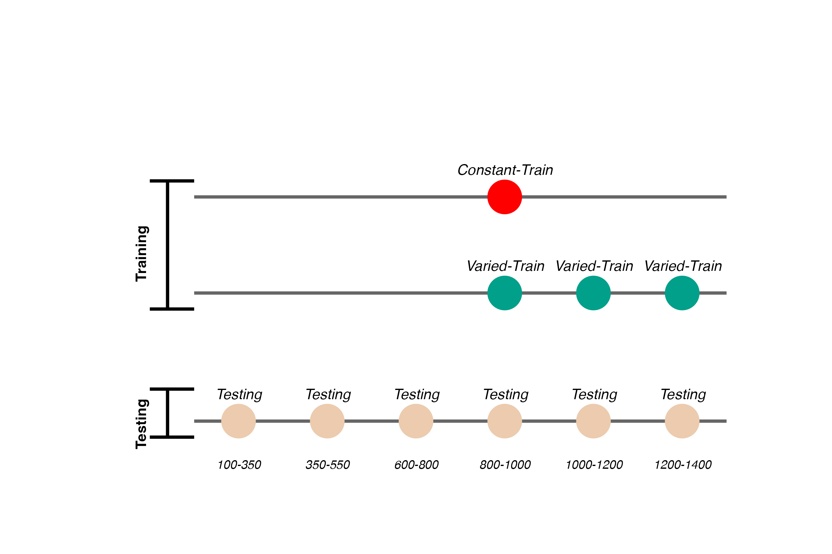

- 156 participants included in final analysis
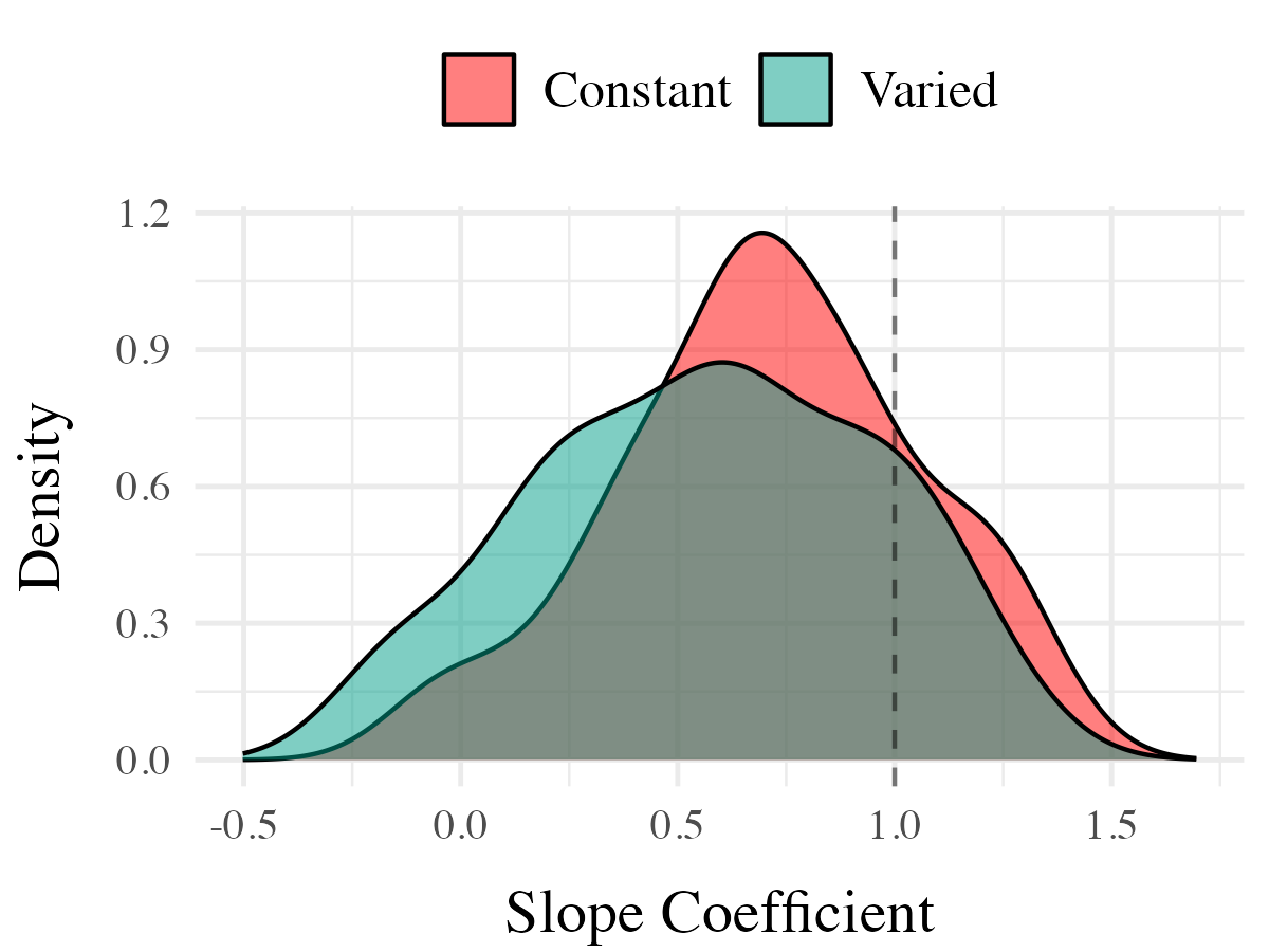
- Varied group trains from 3 “velocity bands”, constant group from 1
- Both groups complete same total number of training trials
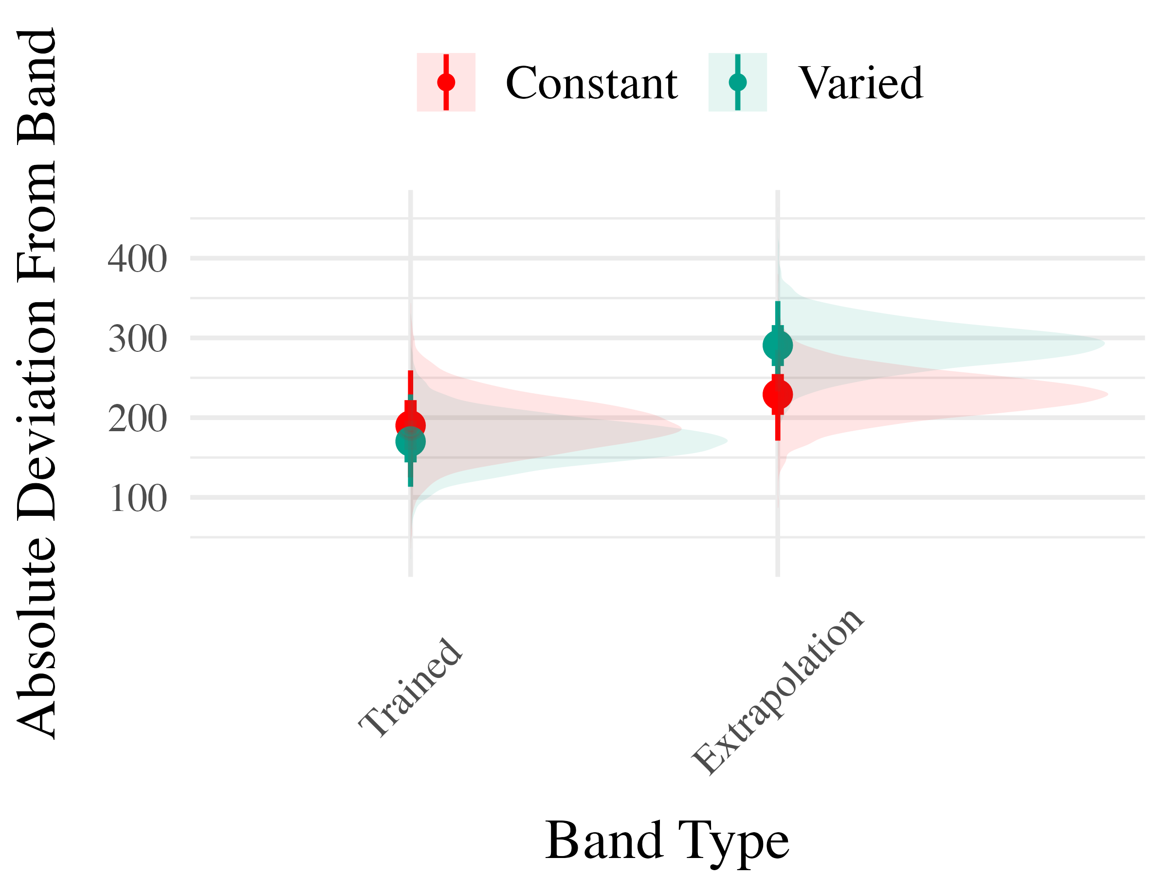
Project 2 - Experiment 1 Results
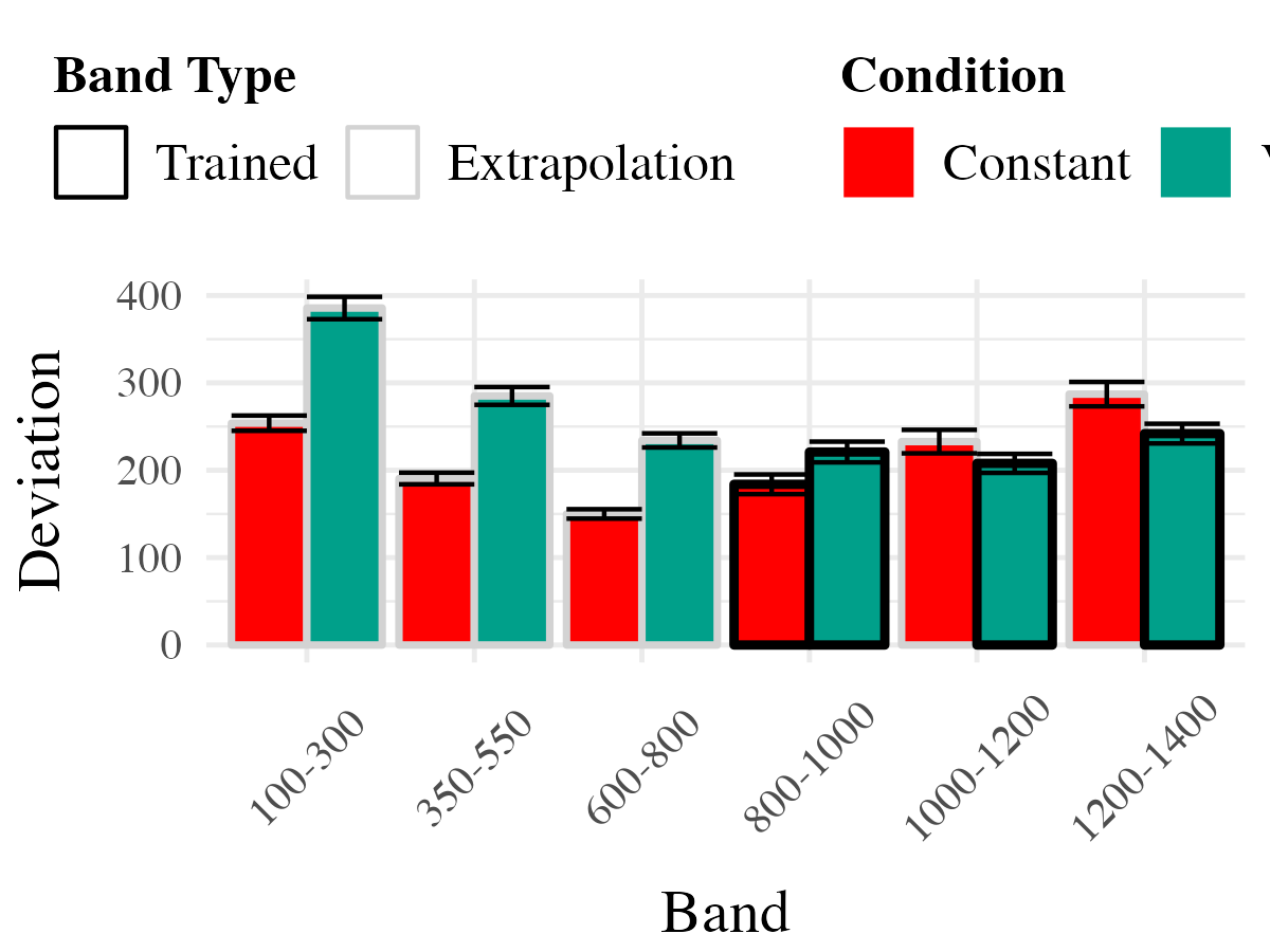
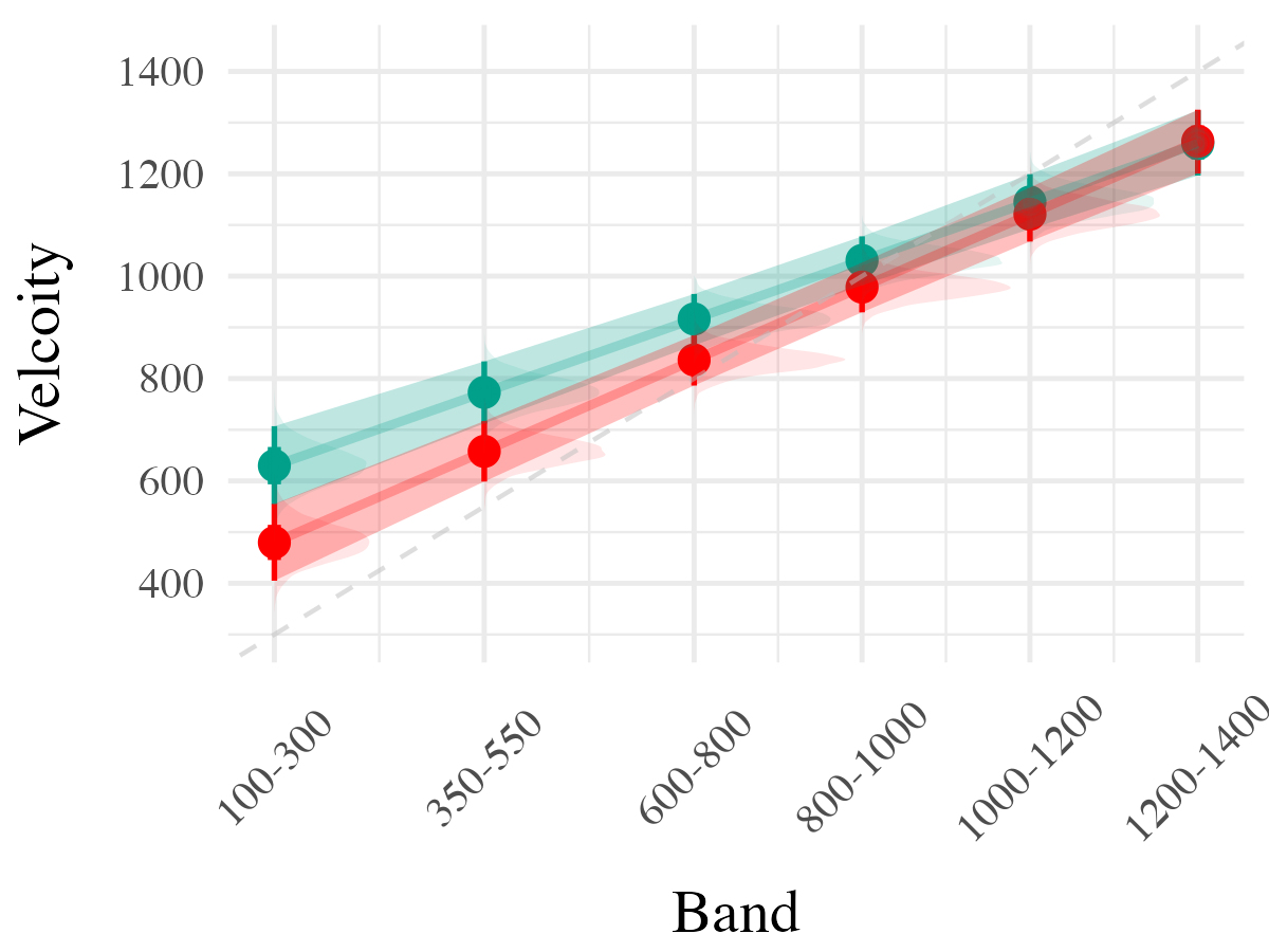
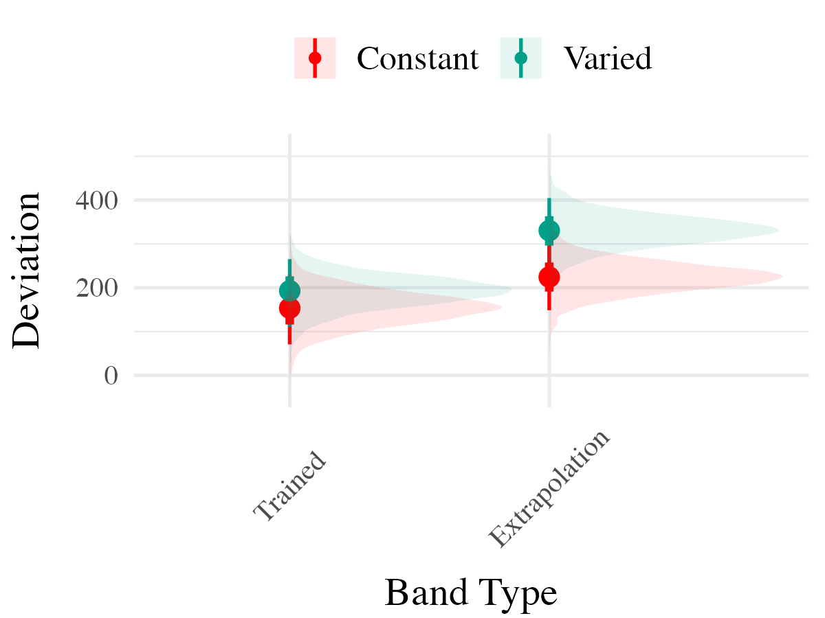
Project 2 - Experiment 2 Design
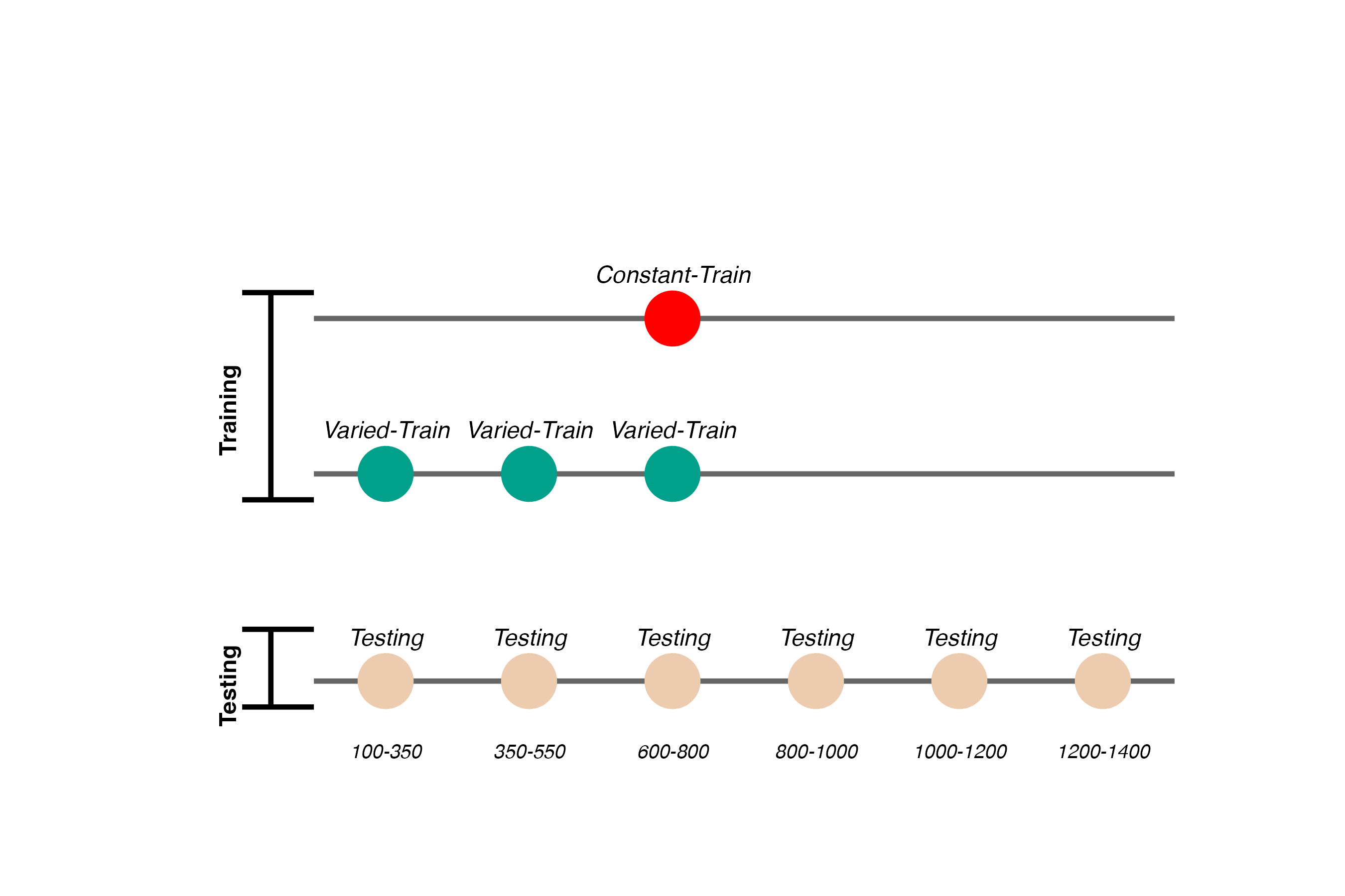

- Training and Testing bands are in reversed order, relative to Experiment 1
- 110 participants included in final analysis
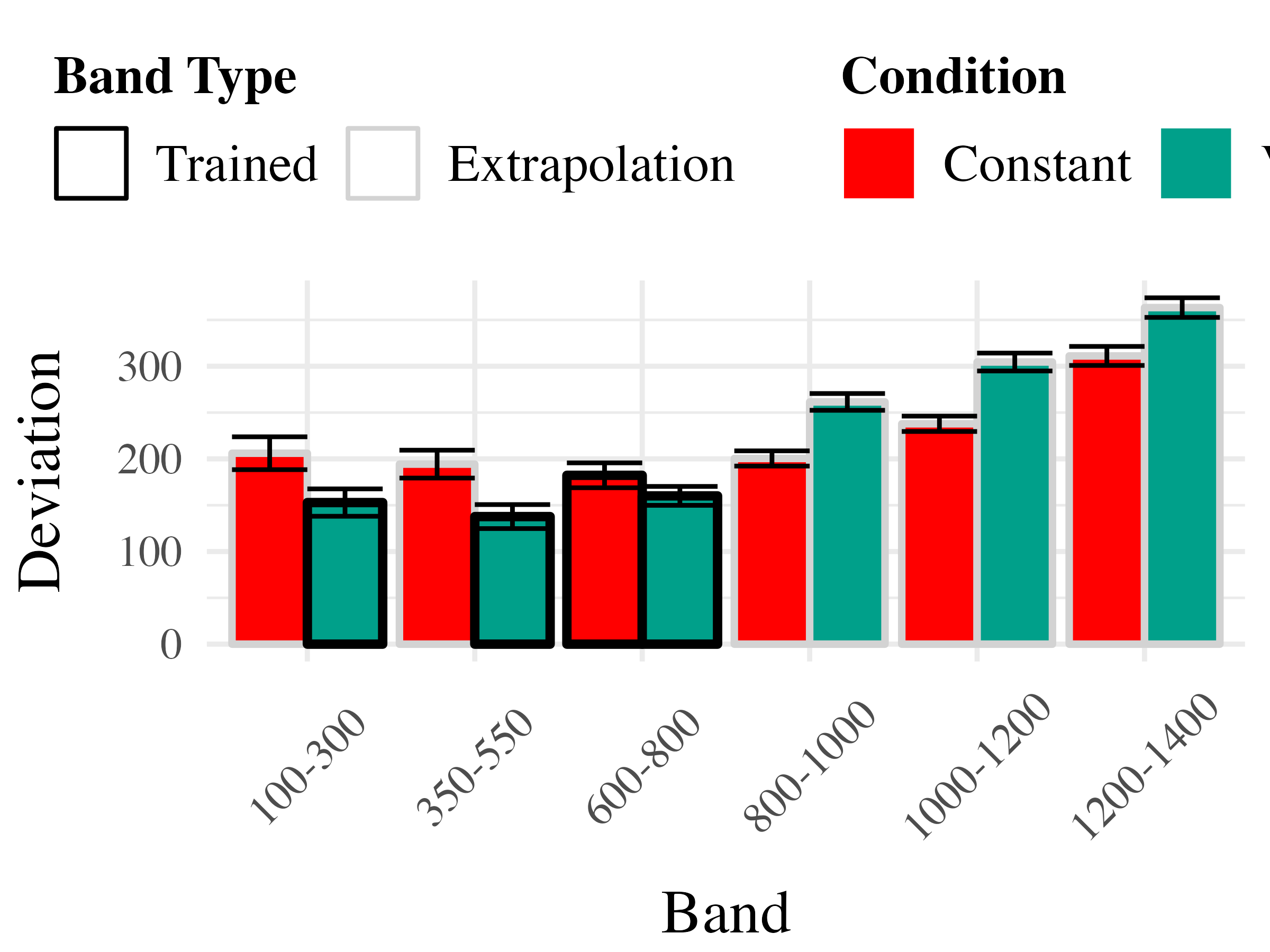
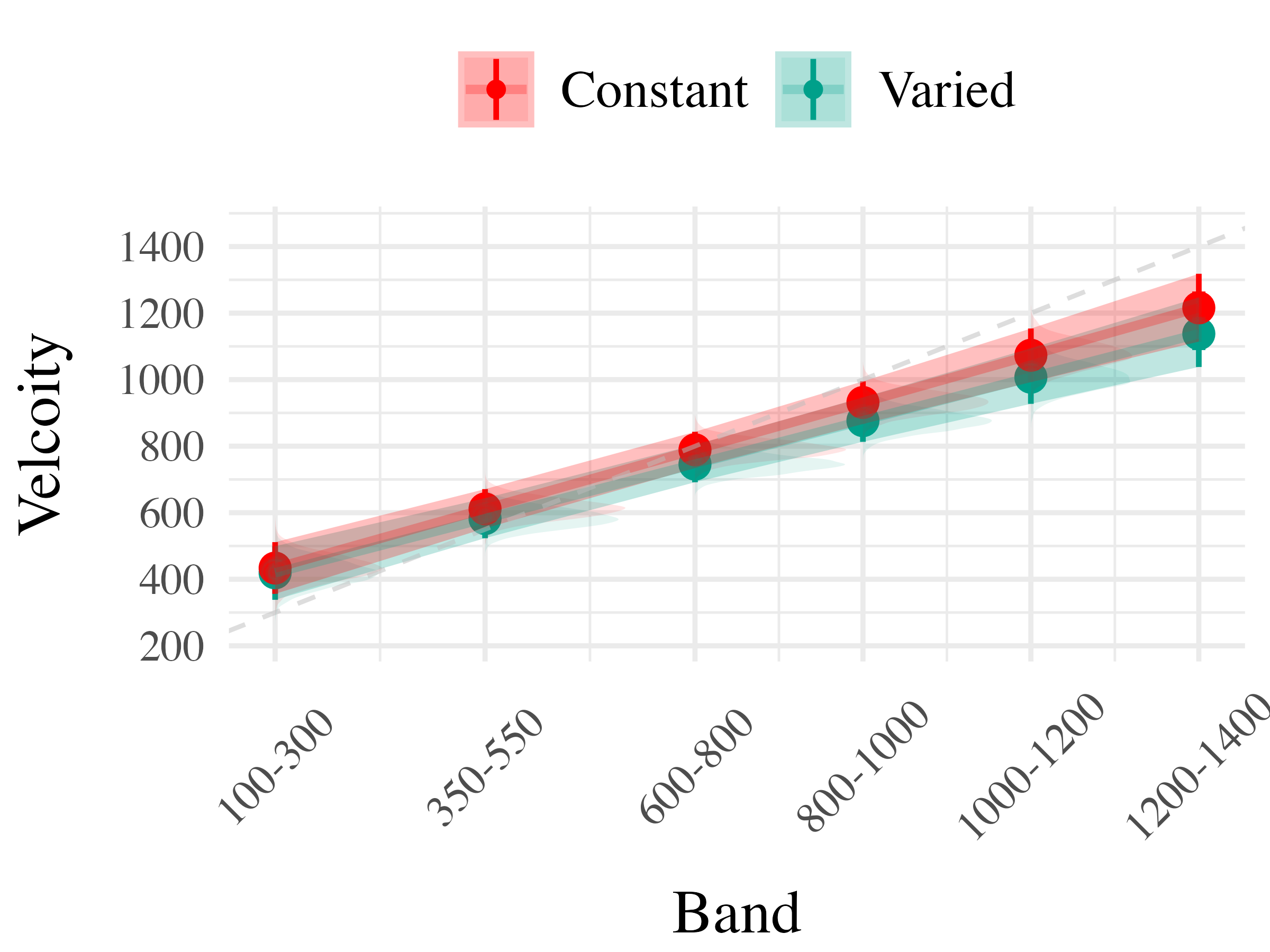
Project 2 - Experiment 2 Results
Project 2 - Experiment 3
- Ordinal Feedback
- directional feedback indicating too high, too low, or correct
- Both Original (Experiment 1), and reverse (Experiment 2) orders included
- 195 participants included in final analysis
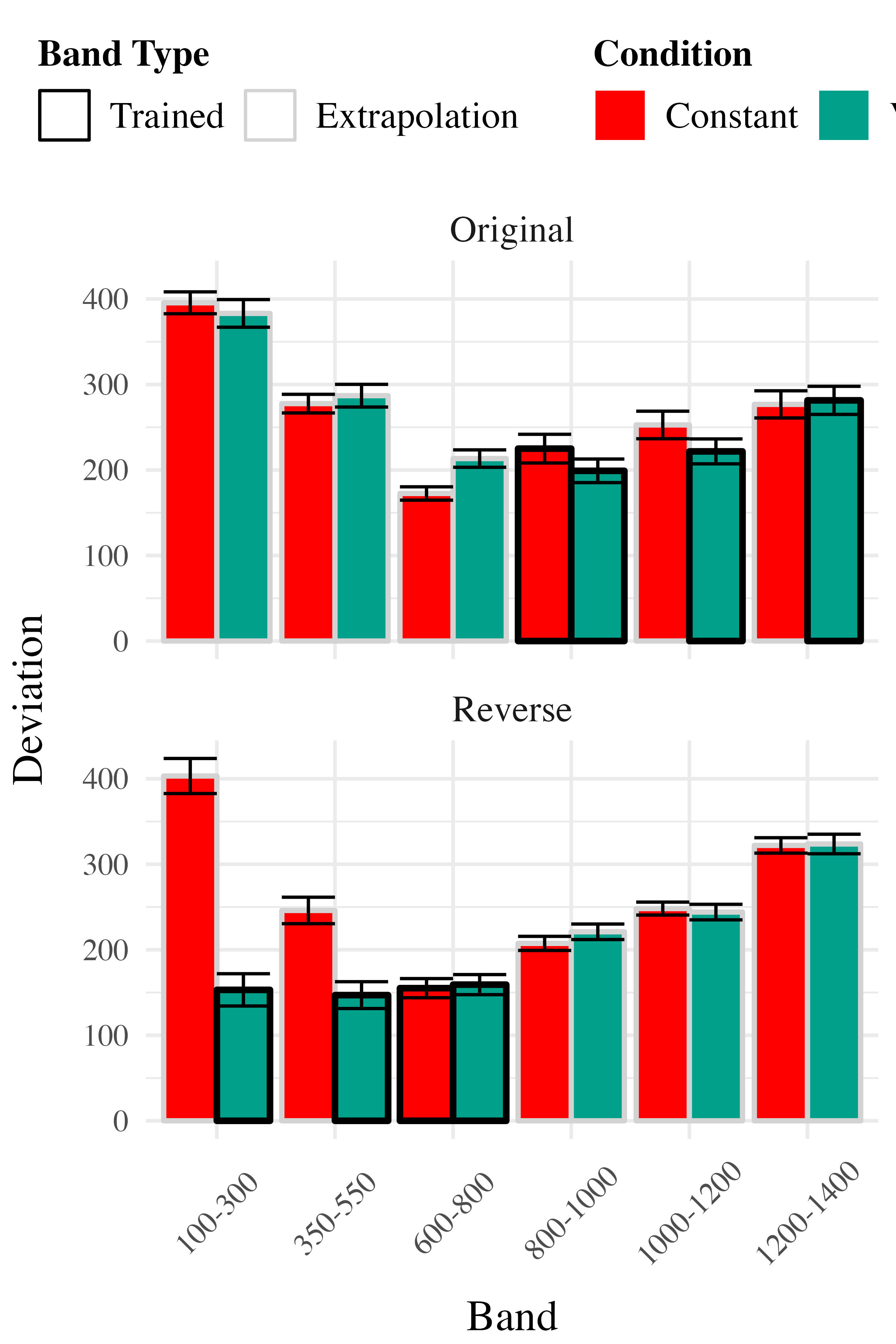
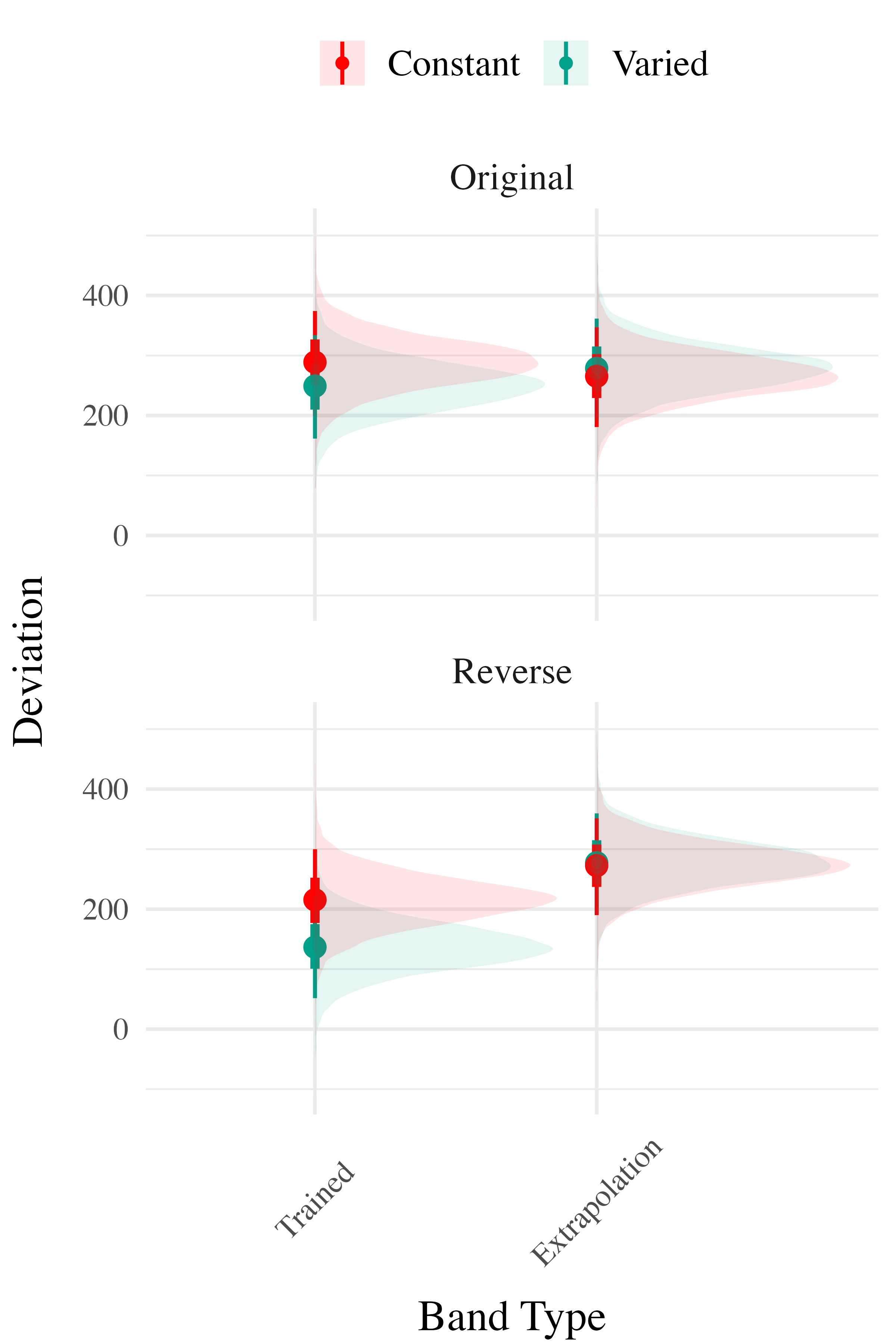
Project 2 - Experiment 3 Results
Experiment 3 - Accuracy
Experiment 3 - Discrimination
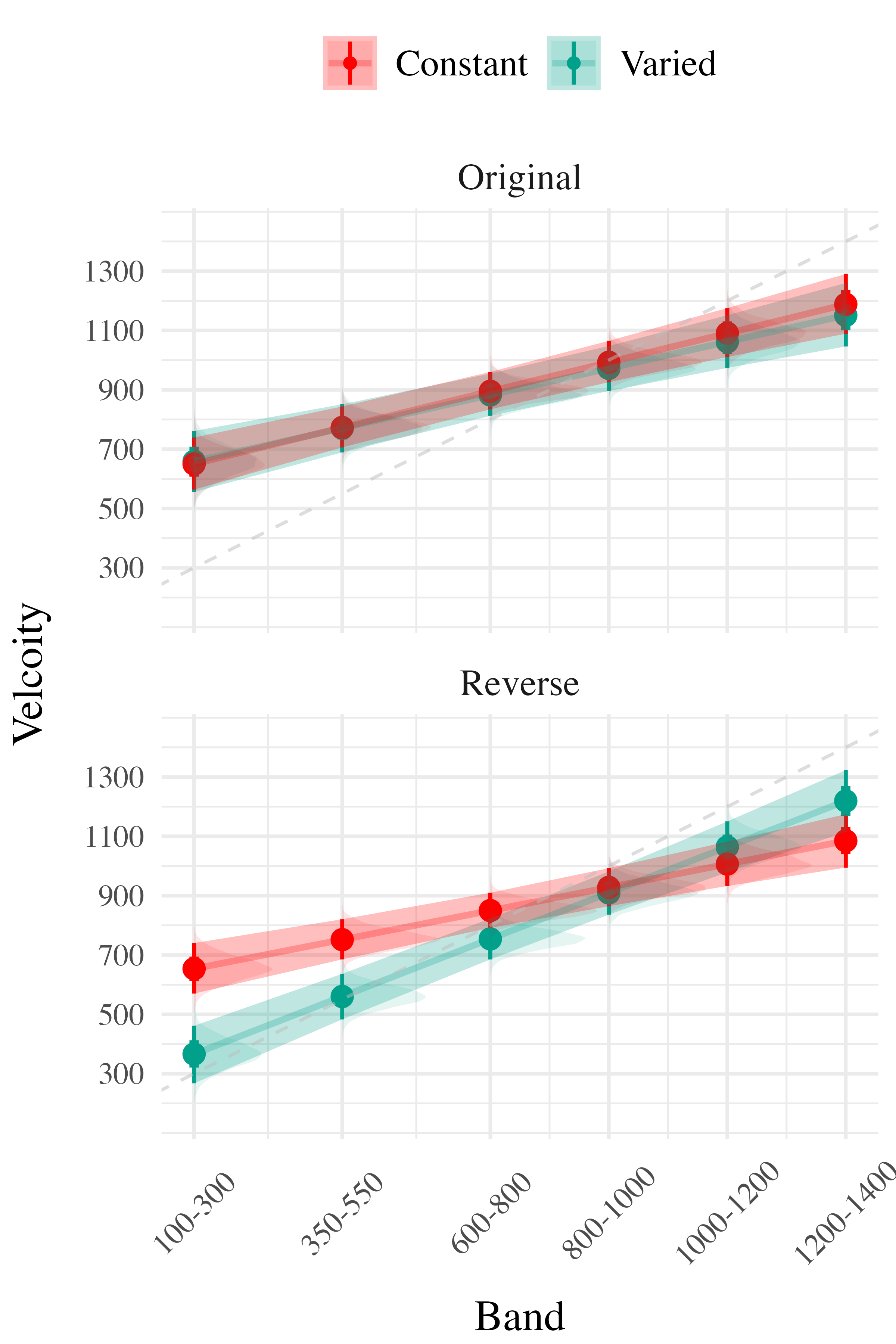
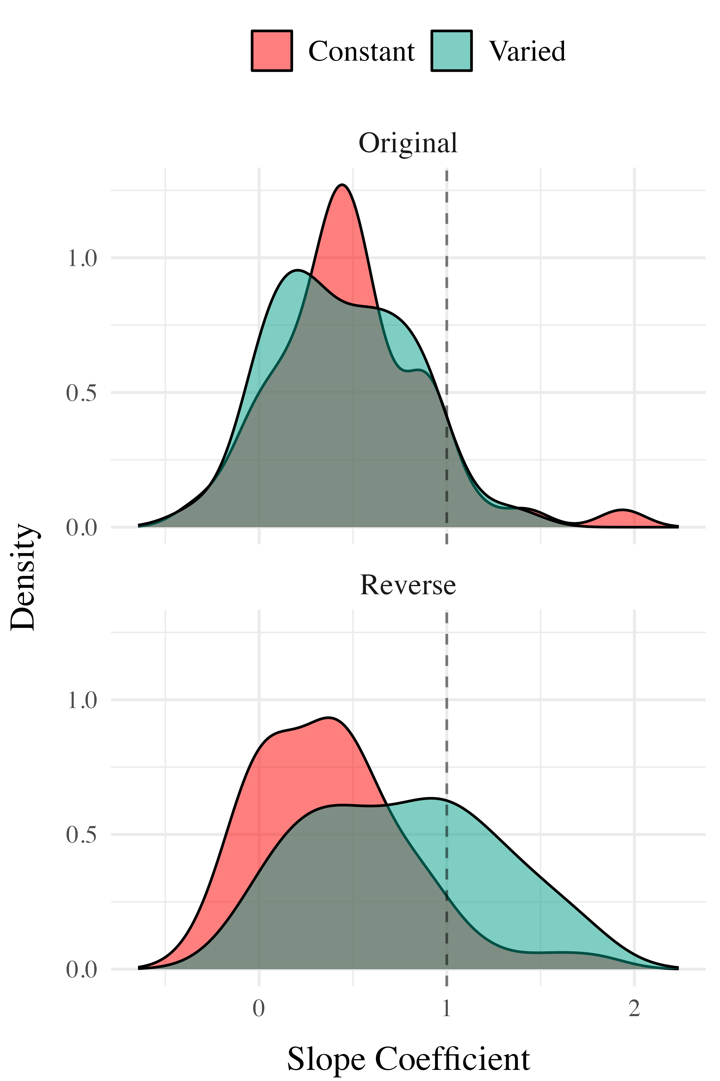
Project 2 - Computational Modeling
The Associative Learning Model ALM
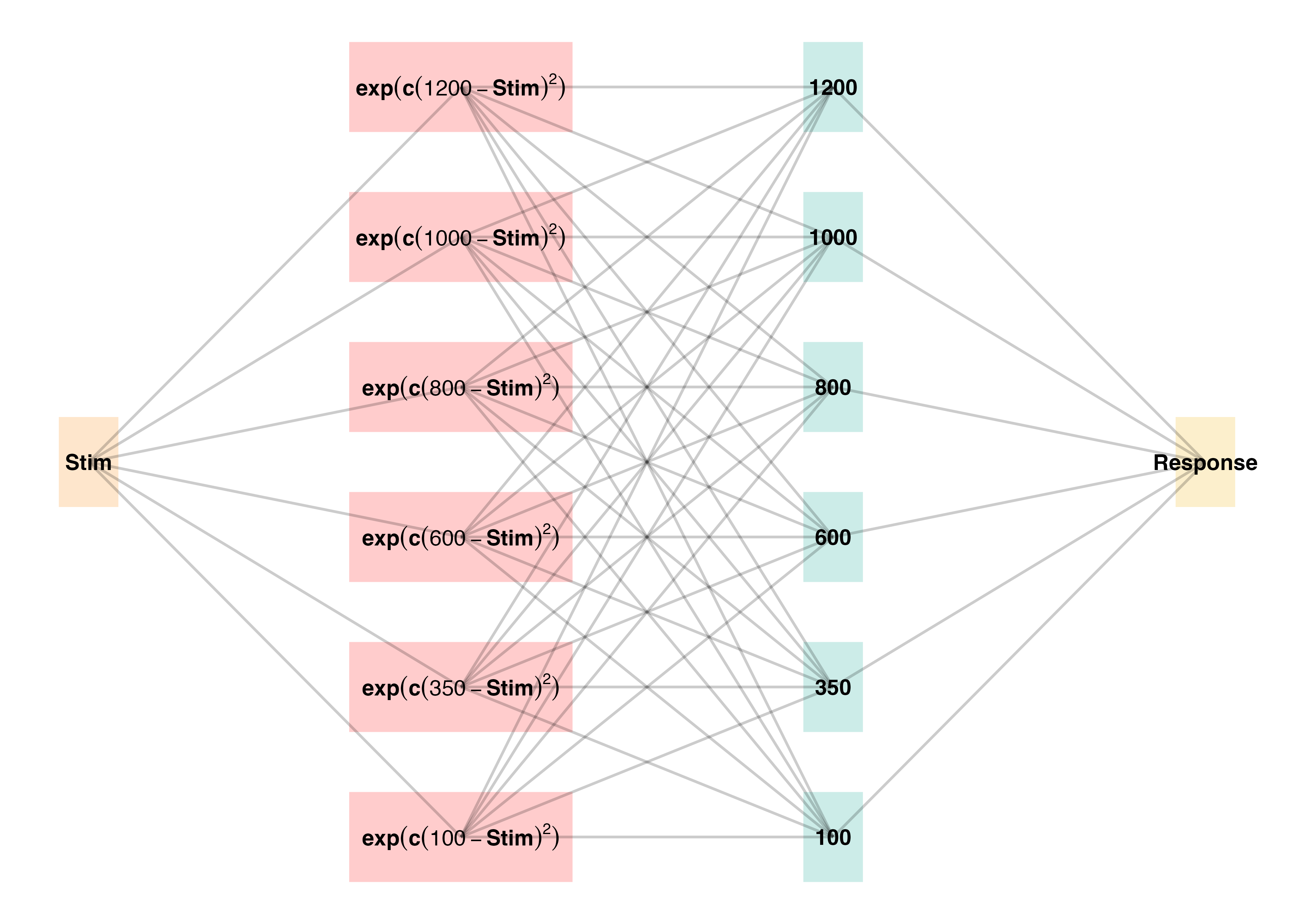
- Two layer network - adapted from ALCOVE (Kruschke (1992))
- Input layer node for each stimulus, output node for each response
- Input nodes activate as a function of their Gaussian similarity to the stimulus
- Weights udpated via delta rule - error driven learning
- Provides good account of human learning data, and interpolation performance, but struggles with extrapolation (DeLosh et al., 1997)
Extrapolation - Association Model (EXAM)
- Extension to ALM to account for human extrapolation behavior
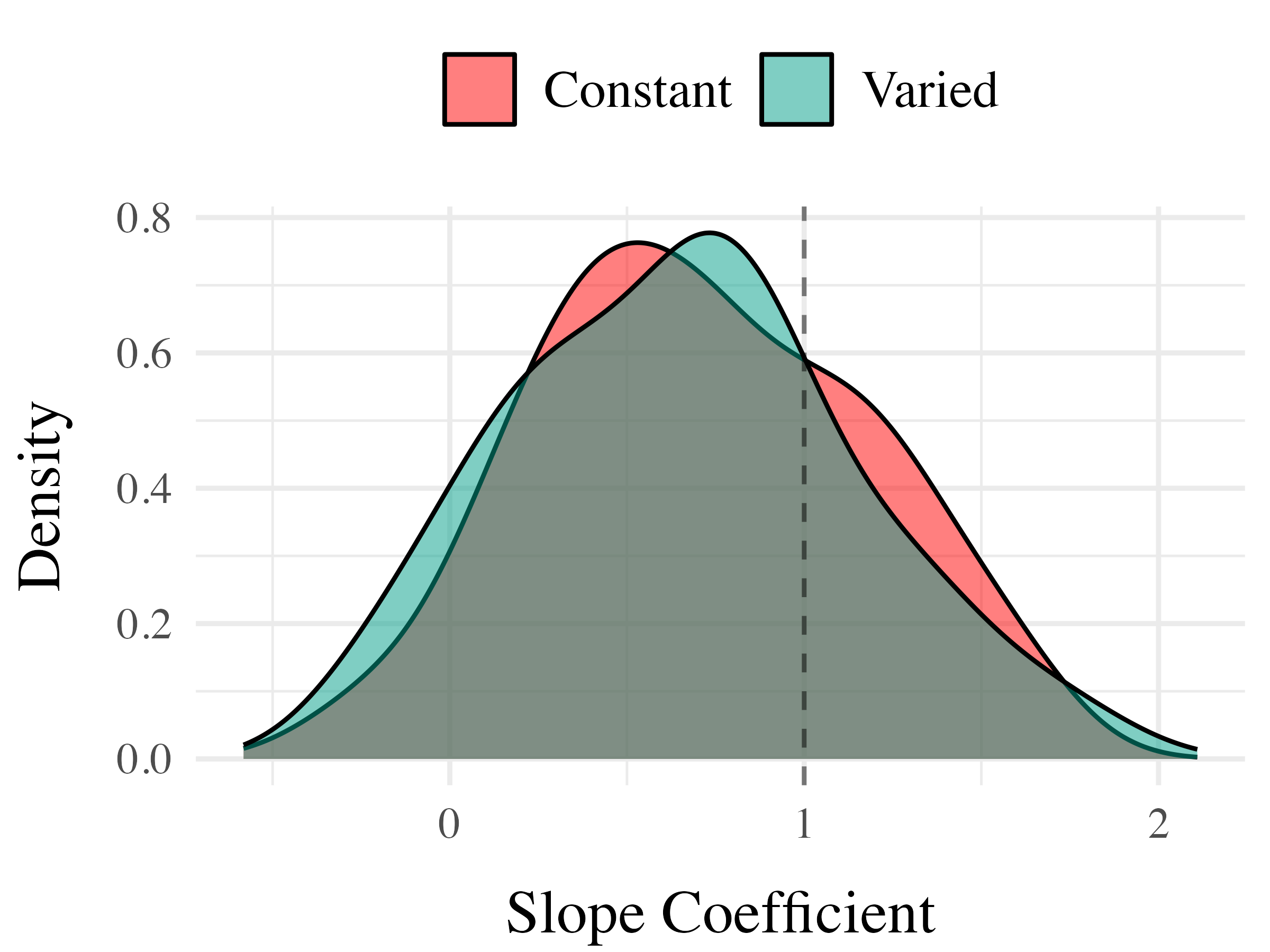
- When a novel stimulus is presented, EXAM assumes the nearest 2-3 prior examples are retrieved, and used to compute a slope
- The slope is used to adjust the ALM response
| EXAM Response Generation | ||
|---|---|---|
| Slope Computation | \(S = \frac{m(X_{1})-m(X_{2})}{X_{1}-X_{2}}\) | Slope value, \(S\) computed from nearest training instances |
| Response | \(E[Y|X_i] = m(X_i) + S \cdot [X - X_i]\) | Final EXAM response is the ALM response for the nearest training stimulus, \(m(X_i)\), adjusted by local slope \(S\). |
Project 2 - Model Fitting Procedure
Approximate Bayesian Computation (ABC)
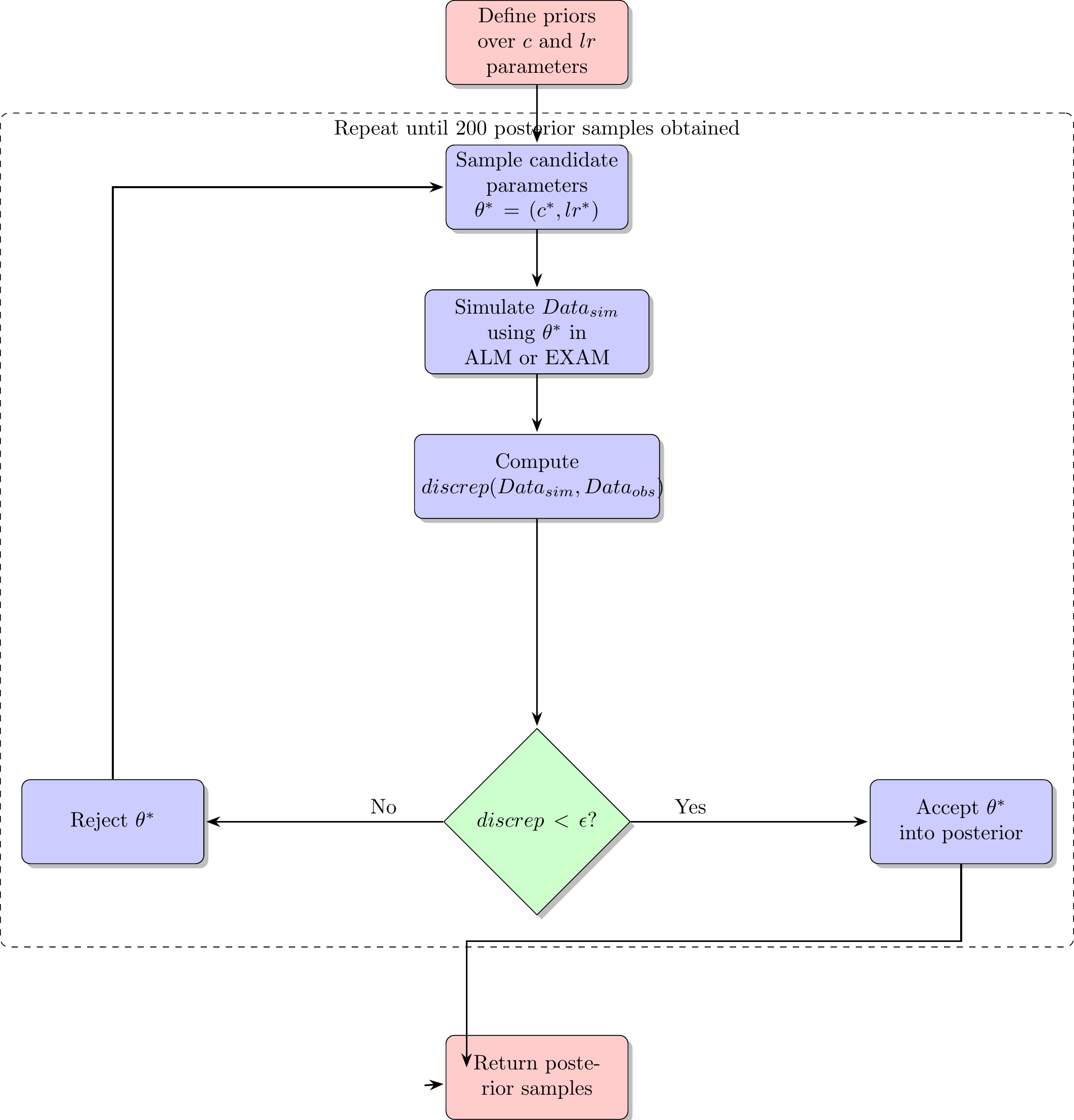
- simulation based parameter estimation (Kangasrääsiö et al., 2019; Turner & Van Zandt, 2012)
- Useful for models with unknown likelihood functions (e.g. many neural network and drift diffusion models)
- full distribution of plausible model predictions for each participant
Project 2 - Model Fitting Procedure
Model Fitting Approach
- Two parameters for both ALM and EXAM
- generalization parameter: \(c\)
- learning rate parameter: \(lr\)
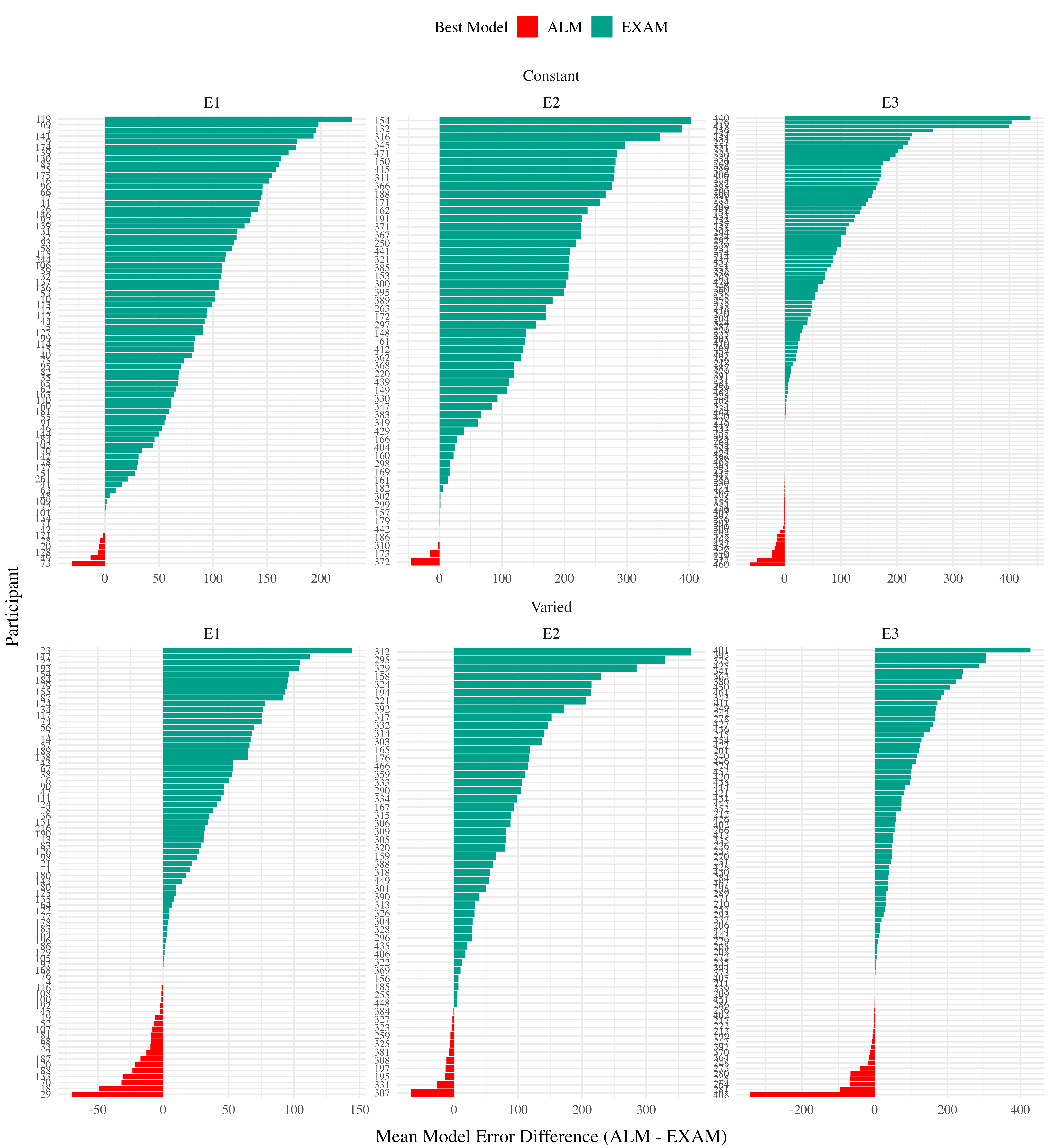
- ALM and EXAM fit separately to each individual participant
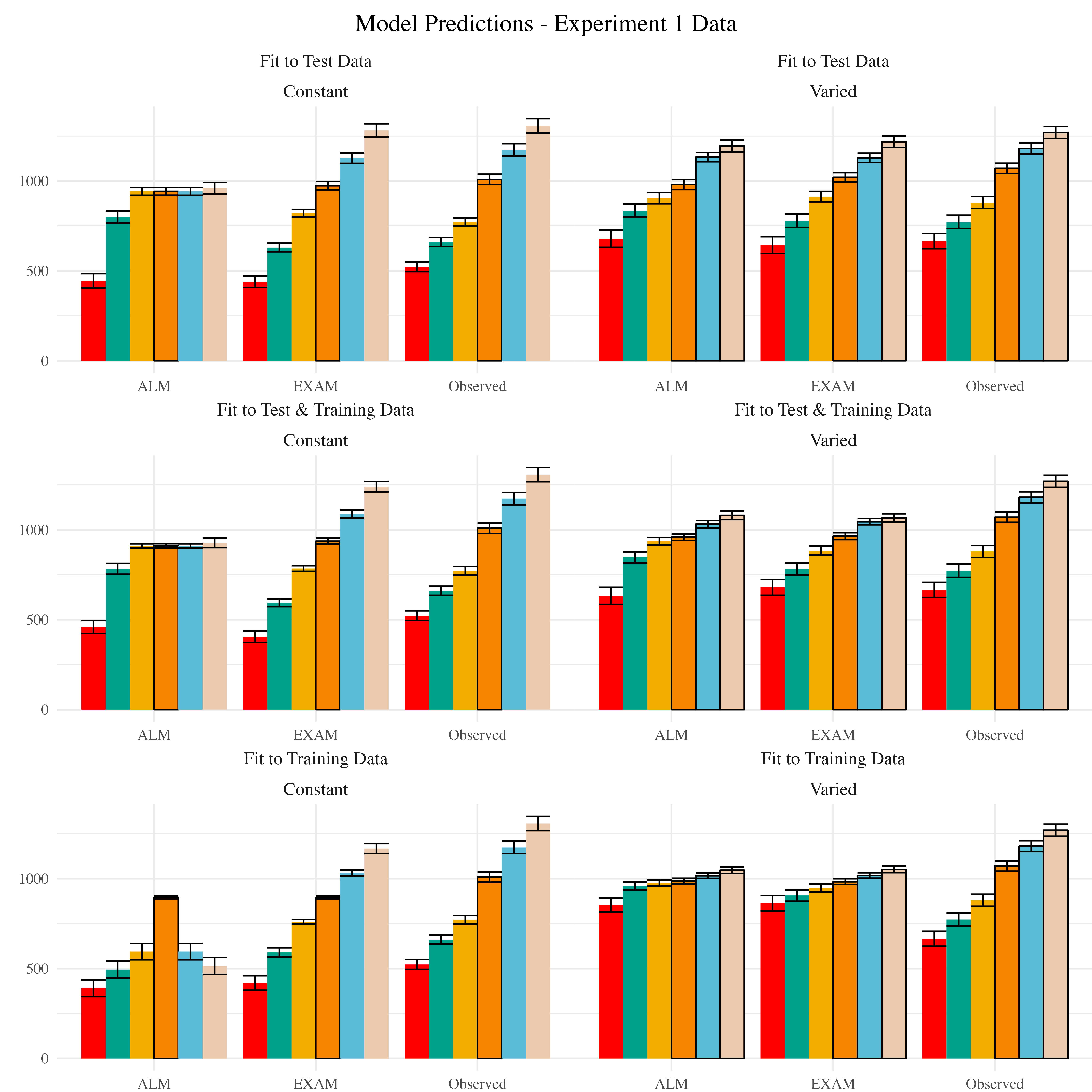
- Rejection based ABC used to obtain 200 posterior samples, per participant, per model
- i.e. 200 plausible values of \(c\) and \(lr\)
- All models fit with three different approaches
- Fit to only the training data
- Fit to both training and testing data
- Fit to only testing data
Modelling Results
Posterior Predictive Distribution
Modelling Results
Best fitting models per participant
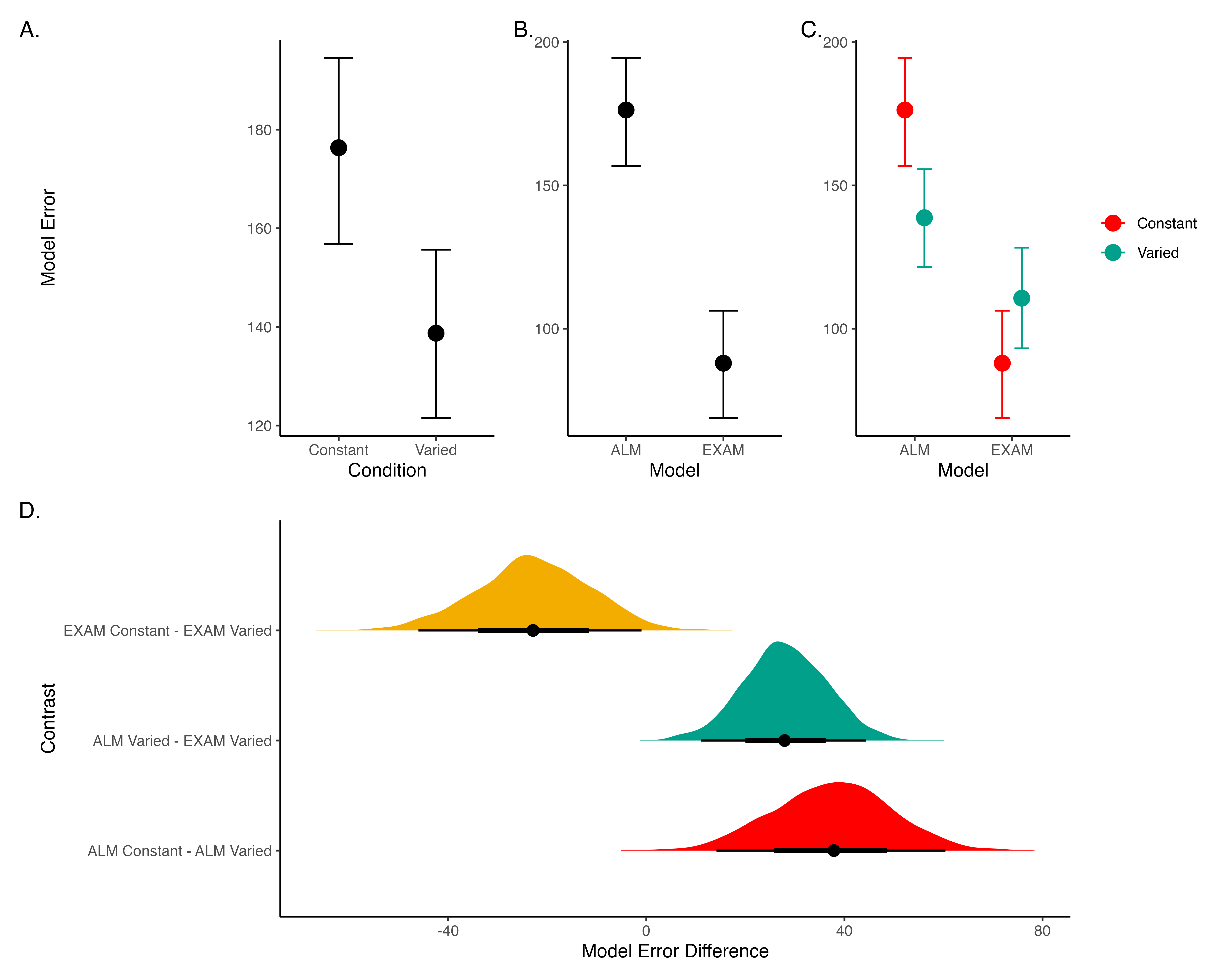
Model Comparison - Experiment 1
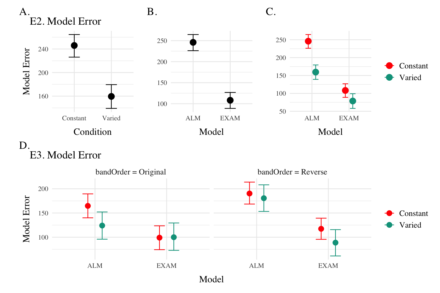
Model Comparison - Experiment 2 and 3
General Discussion
Summary
- Project Comparison:
- HTT (Project 1): Varied training led to superior testing performance.
- HTW (Project 2): Varied training led to poorer performance.
- Key Findings:
- HTT: Varied group outperformed constant group in both training and testing.
- HTW: Varied group exhibited poorer performance across training and testing stages.
- Modeling Approaches:
- HTT: IGAS model quantifies similarity between training and testing conditions.
- HTW: ALM and EXAM models fit to individual participant data.
Project Comparison
- Task Differences:
- HTT:
- Complex parabolic trajectory.
- Both x and y velocities relevant.
- Perceptually salient varied conditions.
- HTW:
- Simple 1D force mapping.
- Only x velocity relevant.
- Less perceptually salient varied conditions.
- HTT:
- Task Complexity:
- HTT: More complex task space with irregularities.
- HTW: Smooth, linear mapping between velocity and feedback.
Conclusion
- Task-specific characteristics are crucial in determining the benefits of varied training.
- Combining empirical research with computational modeling enhances understanding of learning and generalization.
References
Bjork, E. L., & Bjork, R. A. (2011). Making things hard on yourself, but in a good way: Creating desirable difficulties to enhance learning. Psychology and the Real World: Essays Illustrating Fundamental Contributions to Society, 2, 59–68.
DeLosh, E. L., McDaniel, M. A., & Busemeyer, J. R. (1997). Extrapolation: The Sine Qua Non for Abstraction in Function Learning. Journal of Experimental Psychology: Learning, Memory, and Cognition, 23(4), 19. https://doi.org/10.1037/0278-7393.23.4.968
Gorman, T. E., & Goldstone, R. L. (2022). An instance-based model account of the benefits of varied practice in visuomotor skill. Cognitive Psychology, 137, 101491. https://doi.org/10.1016/j.cogpsych.2022.101491
Guadagnoli, M. A., & Lee, T. D. (2004). Challenge Point: A Framework for Conceptualizing the Effects of Various Practice Conditions in Motor Learning. Journal of Motor Behavior, 36(2), 212–224. https://doi.org/10.3200/JMBR.36.2.212-224
Kangasrääsiö, A., Jokinen, J. P. P., Oulasvirta, A., Howes, A., & Kaski, S. (2019). Parameter Inference for Computational Cognitive Models with Approximate Bayesian Computation. Cognitive Science, 43(6), e12738. https://doi.org/10.1111/cogs.12738
Kerr, R., & Booth, B. (1978). Specific and varied practice of motor skill. Perceptual and Motor Skills, 46(2), 395–401. https://doi.org/10.1177/003151257804600201
Kruschke, J. K. (1992). ALCOVE: An exemplar-based connectionist model of Category Learning. Psychological Review, 99(1). https://doi.org/10.1037/0033-295X.99.1.22
Schmidt, R. A. (1975). A schema theory of discrete motor skill learning. Psychological Review, 82(4), 225–260. https://doi.org/10.1037/h0076770
Turner, B. M., & Van Zandt, T. (2012). A tutorial on approximate Bayesian computation. Journal of Mathematical Psychology, 56(2), 69–85. https://doi.org/10.1016/j.jmp.2012.02.005
Extras
Manuscript
ALM
| ALM Response Generation | ||
|---|---|---|
| Input Activation | \(a_i(X) = \frac{e^{-c(X-X_i)^2}}{\sum_{k=1}^M e^{-c(X-X_k)^2}}\) | Input nodes activate as a function of Gaussian similarity to stimulus |
| Output Activation | \(O_j(X) = \sum_{k=1}^M w_{ji} \cdot a_i(X)\) | Output unit \(O_j\) activation is the weighted sum of input activations and association weights |
| Output Probability | \(P[Y_j|X] = \frac{O_j(X)}{\sum_{k=1}^M O_k(X)}\) | The response, \(Y_j\) probabilites computed via Luce’s choice rule |
| Mean Output | \(m(X) = \sum_{j=1}^L Y_j \cdot \frac{O_j(x)}{\sum_{k=1}^M O_k(X)}\) | Weighted average of probabilities determines response to X |
| ALM Learning | ||
| Feedback | \(f_j(Z) = e^{-c(Z-Y_j)^2}\) | feedback signal Z computed as similarity between ideal response and observed response |
| magnitude of error | \(\Delta_{ji}=(f_{j}(Z)-o_{j}(X))a_{i}(X)\) | Delta rule to update weights. |
| Update Weights | \(w_{ji}^{new}=w_{ji}+\eta\Delta_{ji}\) | Updates scaled by learning rate parameter \(\eta\). |
EXAM
| EXAM Response Generation | ||
|---|---|---|
| Instance Retrieval | \(P[X_i|X] = \frac{a_i(X)}{\sum_{k=1}^M a_k(X)}\) | Novel test stimulus \(X\) activates input nodes \(X_i\) |
| Slope Computation | \(S = \frac{m(X_{1})-m(X_{2})}{X_{1}-X_{2}}\) | Slope value, \(S\) computed from nearest training instances |
| Response | \(E[Y|X_i] = m(X_i) + S \cdot [X - X_i]\) | Final EXAM response is the ALM response for the nearest training stimulus, \(m(X_i)\), adjusted by local slope \(S\). |
Comparison {.scrollable .unnumbered .unlisted, .smaller}
| Dimension | HTT (Project 1) | HTW (Project 2) |
|---|---|---|
| Task Description | Projectile launching to hit a target | Projectile launching to hit wall at a specific velocity |
| Task Complexity | More complex parabolic trajectory, both x and y velocities relevant to outcome | Simpler 1D mapping of force to outcome. Only x velocity is relevant. |
| Task Space | More complex: xy velocity combinations closer to the solution space may still result in worse feedback due to striking the barrier. | Simpler: smooth, linear mapping between velocity and feedback. |
| Perceptual salience of Varied Conditions | Varied conditions (# of throwing distances) are perceptually distinct, i.e. salient differences in distance between launching box and target. | Varied conditions (# of velocity bands) are less salient - only difference is the numeral displayed on screen. |
| Testing Feedback | Testing always included feedback | Primary testing stage had no feedback. |
| Potential for Learning during Testing | Limited potential for learning during testing due to feedback. | Some potential for learning during no-feedback testing by observing ball trajectory. |
| Training Experience | Varied group gets half as much experience on any one position as the constant group. | Varied group gets 1/3 as much experience on any one velocity band as the constant group. |
| Testing Structure | Random interleaving of trained/transfer testing distances. | Blocked structure, separately testing trained vs extrapolation testing bands. |